How to Think About Asymptotic Times in Transformer Forward Passes

This post is written for someone who has read the standard "roofline model" tutorials, can derive 2mnk for a GEMM, and now wants to actually predict, and then profile, a transformer training step on a real cluster. It starts from where the textbook stops and builds up an iteration-time predictor operator by operator. It then looks at two real profiles of an 18B-active MoE model on 512 B200s and sees how predictions interact with reality, especially the failure modes that appear when pipeline parallelism is in play.

1. Why `max(compute, I/O)` Is Not Enough

The first thing most people learn about hardware performance is the roofline model

T_{op} = max (\frac{F}{F_{peak}}, \frac{B}{β_{HBM}})

where $F$ is FLOPs, $B$ is bytes moved between HBM and on-chip SRAM, $F_{peak}$ is the device peak FLOPs/sec, and $β_{HBM}$ is the HBM bandwidth. The pitch of the roofline is "we're either compute-bound or memory-bound, and the bound that matters is whichever takes longer."

This is a useful mental model, and it is insufficient for three reasons.

Real GEMMs do not run at $F_{peak}$ . A bf16 GEMM on a B200 advertises ~2.25 PFLOP/s, but at production shapes you typically see 50–80% of that. The shortfall is real and varies by shape, dtype and library. Calling it "compute-bound" is correct. Calling it "compute-bound at peak" is not.
Non-GEMM ops do not have a single $B$ . A LayerNorm reads the input, computes statistics, and writes the output, which is a roundtrip with three HBM passes, not one. A permutation in MoE dispatch reads and writes the activation twice.
A transformer step is not one op. It is dozens of operators per layer, plus collectives, plus a pipeline bubble, plus a kernel-launch tax, plus an optimizer step. A roofline tells you nothing about how those compose.

So the question actually worth answering is the following. For a given parallel layout $X = (X_{TP}, X_{EP}, X_{CP}, X_{PP}, X_{DP})$ , batch $B$ , and model config $Z$ , what is the iteration time? With that in hand, MFU, memory pressure, and the marginal effect of every knob can all be reasoned about.

The notation below is used throughout, lifted from a more formal performance model.

$b_{w}$ , parameter byte-width (so $2$ for bf16).
$m : = B_{micro} h / X_{CP}$ , local token count on a CP rank (per microbatch, per CP shard).
$d$ , $d_{ff}$ , $d_{head}$ , $G_{q}$ , $G_{k}$ , meaning hidden, MLP-inner, head dim, Q-head count, KV-head count.
$η_{op} \in (0, 1]$ , a measured per-shape efficiency for an op. This is the most important fitted constant, with more on it below.

2. Three Cost Rules: GEMM, HBM, Collective

Instead of one roofline, the model uses three closed-form rules and composes them.

Rule 1, Compute-Bound GEMM

For any matmul with FLOP count $F$ ,

T_{gemm} (F, η) = \frac{F}{F_{peak} η} .

The fitted $η$ absorbs everything the roofline pretends does not exist, including tile-shape efficiency, the fact that the GEMM has low arithmetic intensity at this batch and is partially DRAM-bound, the cost of writing the output, etc. Different GEMMs at different shapes get different $η$ s. In practice you fit one $η$ per named op (qkv, attn_out, mlp_up, mlp_down, router, expert_up, expert_down) at the shapes you actually use, and that is enough.

The reason GEMMs stay pinned to the compute branch even when arithmetic intensity is low is that mixing branches in the model multiplies the prediction error. A GEMM at low intensity is not actually a memory-bandwidth event in the way a LayerNorm is, because the kernel still streams through tensor cores. The slowdown shows up as a smaller $η$ , not as a switch to a different formula.

Rule 2, Bandwidth-Bound HBM Traffic

For norms, RoPE, residuals, GLU activations, top- $K$ , and permutations, the cost is

T_{hbm} (B; c) = \frac{c B}{β_{HBM}} .

The number $c$ counts HBM passes.

Op	Forward $c$	Backward $c$
LayerNorm / RMSNorm	3	5
RoPE	3	3
Residual add	2	3
GLU activation	3	5
Permutation (dispatch + undo)	4	4

Three HBM passes for a forward LayerNorm because you read input, read input again to subtract mean and divide variance, and write the output. The backward needs gradient w.r.t. the input plus gradient w.r.t. weights, hence five. These are not heuristics. They are counts of how many times the tensor crosses the SRAM/HBM boundary. If you have ever wondered why "I optimized my kernel and it got 5% faster," it is because you forgot one of these passes, or your fused kernel collapsed two of them.

Rule 3, Collectives

Ring reduce-scatter / all-gather over $P$ ranks for a tensor of size $S$ bytes costs

T_{ring} (S, P) = (P - 1) t_{link} + \frac{(P - 1) S / P}{α_{nccl} (S) β_{link}} .

The textbook usually skips two notes.

$α_{nccl} (S)$ is the NCCL protocol efficiency. It is not a constant. NCCL picks LL / LL128 / Simple based on size thresholds (typically around 32 KB and 1 MB), with $α \in {0.5, 0.7, 0.9}$ . A small collective does not just have higher per-byte cost from latency, it also runs at half the asymptotic bandwidth.
All-to-all has the same algebraic shape but with an inter-node fraction $f_{inter} = (n_{node} - 1) / n_{node}$ multiplying the bandwidth term whenever the EP group spans nodes. This is the single largest correction to the bandwidth-only model for MoE workloads.

The shorthand $T_{AG}, T_{RS}, T_{A2A}$ is used for the relevant ring evaluations.

3. Walking Through an Attention Block

Now add up an attention block, forward only. This is the pattern. Commit it to memory and the rest of the model is just variations.

Op	Cost
Pre-attn norm	$T_{hbm} (m d b_{w}; 3)$
RoPE	$T_{hbm} (m d b_{w}; 3)$
Pre-attn all-gather	$T_{AG} (m d b_{w}, X_{TP})$
QKV proj	$T_{gemm} (2 m d (G_{q} + 2 G_{k}) d_{head} / X_{TP}; η_{qkv})$
SDPA	see below
Attn-out proj	$T_{gemm} (2 m d^{2} / X_{TP}; η_{out})$
Post-attn reduce-scatter	$T_{RS} (m d b_{w}, X_{TP})$
Post-attn residual	$T_{hbm} (m d b_{w}; 2)$

SDPA at FlashAttention arithmetic intensity is treated as compute-bound,

F_{sdpa} = \frac{G_{q}}{X_{TP}} (2 m d_{head} h + 2 h^{2} d_{head}), T_{sdpa} = \frac{F_{sdpa}}{F_{peak} η_{sdpa}} .

There are a few things to internalize from this table.

The "all-gather → GEMM → GEMM → reduce-scatter" pair flanking attention is the sequence-parallel TP pattern. The collectives are not a tax on top of TP. They are TP. If $X_{TP} = 1$ those terms vanish.
The QKV FLOP count carries $(G_{q} + 2 G_{k}) d_{head}$ rather than $3 d$ . For grouped-query attention with $G_{k} ≪ G_{q}$ , this is materially cheaper than the naive $3 d$ count would predict.
Norms, RoPE, residual all live on the bandwidth branch. They look small per-op, but on B200 with bf16 they sum to a non-trivial fraction of attention-block time precisely because $β_{HBM}$ has not scaled as fast as $F_{peak}$ .

4. Dense MLP Block

The dense MLP block is two GEMMs, two collectives, and two HBM ops.

\begin{aligned} T_{MLP up} & = T_{gemm} (2 m d (2 d_{ff}) / X_{TP}; η_{up}), \\ T_{MLP down} & = T_{gemm} (2 m d_{ff} d / X_{TP}; η_{down}) . \end{aligned}

The factor of two on $d_{ff}$ is GLU geometry, where a single fused matmul produces gate-and-up, doubling the output dimension. Drop it for plain MLPs. Flanking ops are pre-MLP norm, pre-MLP all-gather, post-MLP reduce-scatter, and post-MLP residual, the same way attention flanks.

5. The MoE Block, Where the Model Gets Interesting

The MoE block replaces the dense MLP with router, dispatch, expert GEMMs, and combine. Let $E_{loc} = E / X_{EP}$ (per-rank expert count), $c_{exp}$ the padded expert capacity in tokens per local expert, and $d_{expert} = d_{ff} / G$ where $G$ is the granularity.

Op	Cost	Note
Pre-MLP norm	$T_{hbm} (m d b_{w}; 3)$
Router GEMM	$T_{gemm} (2 m d E; η_{rtr})$
Top- $K$	$m E b_{w} / τ_{topk}$	bandwidth-bound, device-fitted $τ$
Permutation	$T_{hbm} (m d b_{w}; 4)$	permute + unpermute
Pre-MLP A2A	$T_{A2A} (E_{loc} c_{exp} d b_{w} / X_{TP}, X_{EP})$	dispatch
Pre-MLP AG	$T_{AG} (E_{loc} c_{exp} d b_{w}, X_{TP})$	expert TP
Expert up	$T_{gemm} (E_{loc} \cdot 2 c_{exp} d (2 d_{expert}) / X_{TP}; η_{eu})$	GLU geometry
GLU activation	$T_{hbm} (E_{loc} c_{exp} d_{expert} b_{w}; 3)$
Expert down	$T_{gemm} (E_{loc} \cdot 2 c_{exp} d_{expert} d / X_{TP}; η_{ed})$
Post-MLP RS	$T_{RS} (E_{loc} c_{exp} d b_{w}, X_{TP})$	expert TP
Post-MLP A2A	$T_{A2A} (E_{loc} c_{exp} d b_{w} / X_{TP}, X_{EP})$	combine
Post-MLP residual	$T_{hbm} (m d b_{w}; 2)$

Two things are easy to get wrong here.

The router is three operators, not one. People casually say "the router" and then handwave a $T_{gemm}$ for it. But the router is three pieces.

a small GEMM into $E$ logits (compute-bound, but at tiny $η$ because the inner dim is small),
a top- $K$ kernel that runs at a device-fitted element throughput $τ_{topk}$ (bandwidth-bound, sometimes surprisingly slow), and
a permutation that reads-and-writes the activation twice.

That third piece, the permute/unpermute, is what the bandwidth-only model usually misses. In MoE traces it shows up as a fat block of memcpy/gather/scatter kernels that you would not naively account for.

Dispatch all-to-all carries an inter-node fraction. $T_{A2A}$ is the term that usually dominates an MoE block when EP spans nodes. If you predict using a naive bandwidth-only model that treats all-to-all as a flat $S / β$ , you will under-predict by 1.5–2× on a multi-node EP group. This is the single largest correction relative to a textbook bandwidth model.

6. The Backward Pass Is Not `1.5×`

There is a piece of folklore that says "backward takes about 1.5× forward." Sometimes it is right. More often it is misleading because the composition of where time is spent changes.

The model here is explicit autograd-style, where every forward operator has a paired backward operator with its own cost rule. For a linear layer with input/output dimensions $(k, n)$ , the backward computes both $d X = d Y W^{⊤}$ and $d W = X^{⊤} d Y$ ,

T_{linear,bwd} = T_{gemm} (2 m n k; η_{dX}) + T_{gemm} (2 m n k; η_{dW}) .

So the GEMM cost of backward is exactly $2 \times$ forward in FLOPs (not 1.5×). The bandwidth-bound ops have their own multipliers (see the table in Rule 2, where LayerNorm goes from 3 to 5 and GLU activation from 3 to 5).

The other thing to track is that TP collectives swap direction on the backward pass. A forward all-gather becomes a gradient reduce-scatter and vice versa. The MoE A2A pair swaps analogously, where the dispatch all-to-all on the forward becomes a combine on the backward, and the combine becomes a dispatch.

The reason the 1.5× rule of thumb still works on dense models trained without recompute is that backward ops are at smaller m if activation checkpointing is used, and the ratio of total backward to total forward depends a lot on how much is GEMM vs bandwidth. If most of the forward is bandwidth-bound (small models, short seqs), backward inflates to roughly $5 / 3 \approx 1.67$ . If it is GEMM-dominated (large models, long seqs), backward is closer to 2.0. The 1.5× was a population-mean over a particular regime.

7. The AdamW Step

AdamW maintains, per parameter, fp32 first and second moments (8 bytes per parameter). With Megatron-style distributed optimizer the states are partitioned across $X_{DP}$ , so per-rank optimizer state is $S_{opt} = 8 N_{tot} / X_{DP}$ bytes.

Per-parameter compute is 11 FLOPs,

\begin{aligned} exp_avg & \leftarrow β_{1} exp_avg + (1 - β_{1}) g & (3 FLOPs) \\ exp_avg_sq & \leftarrow β_{2} exp_avg_sq + (1 - β_{2}) g^{2} & (4 FLOPs) \\ θ & \leftarrow θ - η exp_avg / (\sqrt{exp_avg_sq} + ε) & (4 FLOPs) \end{aligned}

Reading and writing optimizer state dominates wall-clock,

T_{opt} = \underset{state R/W}{\underset{⏟}{\frac{2 S_{opt}}{β_{HBM}}}} + \underset{compute}{\underset{⏟}{\frac{11 N_{tot} / X_{DP}}{F_{peak}}}} .

In every measured regime, the bandwidth term wins by an order of magnitude. The compute term is in the formula for completeness. If you ever see optimizer time scale with model FLOPs rather than parameter count, your distributed optimizer is broken.

8. Putting It Together: Iteration Time and MFU

Sum over $L$ layers (each attention+MLP or attention+MoE), then add the non-overlapped parts of the rest of the step:

T_{iter} = L (T_{block,fwd} + T_{block,bwd}) + T_{DP}^{exp} + T_{bub} + T_{opt} + T_{kl} .

The four "extra" terms are where most of the surprise lives.

$T_{DP}^{exp}$ , the exposed portion of the DP all-gather and reduce-scatter for the distributed optimizer. Most modern frameworks overlap most of this with backward. "Exposed" means whatever did not overlap.
$T_{bub}$ , the pipeline bubble. For 1F1B with PP= $X_{PP}$ and $n_{ub}$ microbatches, the canonical bubble fraction is $(X_{PP} - 1) / n_{ub}$ . Interleaved schedules reduce this by a factor proportional to the virtual-stage count.
$T_{opt}$ , covered above.
$T_{kl}$ , the kernel-launch tax. Modeled as $L \cdot κ (X_{TP}, moe, K) \cdot t_{launch}$ where $κ$ counts kernels per block. This term is tiny at large microbatch and catastrophic at small microbatch, as the case studies below show.

Throughput and MFU then follow as

tok/s = \frac{B_{global} h}{T_{iter}}, MFU = \frac{6 N_{act} \cdot tok/s}{N_{dev} F_{peak}} .

The $6 N_{act}$ factor is the Kaplan-style FLOPs/token count for a forward+backward step with active parameters $N_{act}$ . If you forget the "active" qualifier on an MoE model you will over-report MFU by the activation ratio.

9. Case Study: 18B-Active MoE on 512 B200s, GBS=8192

Now a real profile shows what the model gets right and where reality forces extra terms.

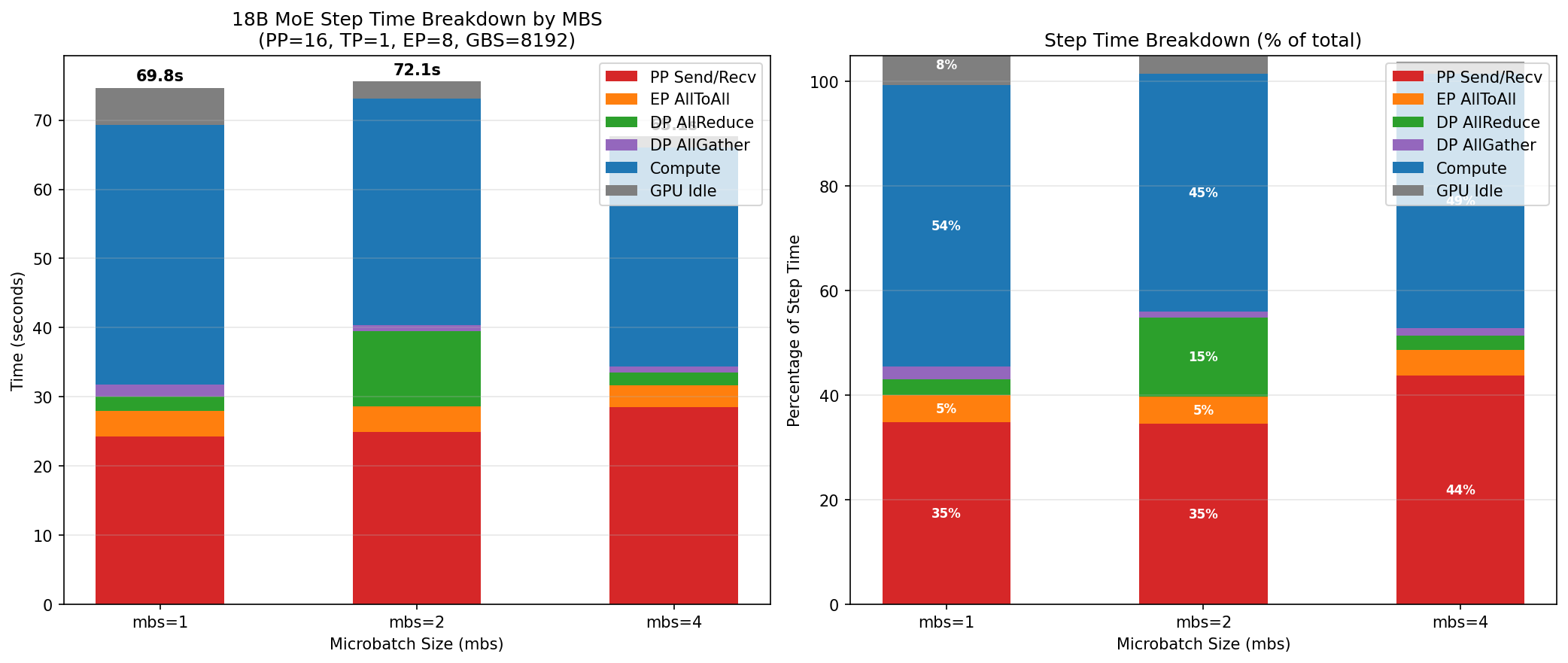
Configuration. 18B active-parameter MoE (1 dense layer + 47 MoE layers), 512 GPUs, PP=16, TP=1, EP=8, DP=32, GBS=8192. Profiled rank 0 of step 106. Three runs sweeping microbatch size $mbs \in {1, 2, 4}$ . Number of microbatches per step is $n_{ub} = GBS / (DP \cdot mbs) = 8192 / (32 \cdot mbs)$ , so 256 / 128 / 64 microbatches respectively.

18B MoE step-time breakdown by microbatch size, GBS=8192
Step time decomposition for the 18B-active MoE at GBS=8192, sweeping mbs ∈ {1, 2, 4}. PP communication is the largest single bucket in every config.

The headline numbers are summarized below.

Bucket	mbs=1	mbs=2	mbs=4
Step duration (s)	69.8	72.1*	65.1
Compute	32.8s (47%)	29.3s (41%)	29.2s (45%)
NCCL	30.3s (43%)	38.9s (54%)	33.0s (51%)
GPU idle	5.3s (7.6%)	2.4s (3.4%)	1.6s (2.4%)
GPU kernel events	383k	182k	94k

*mbs=2 includes an 8.7s straggler AllReduce. Without it, ≈ 63.5s.

Now decompose the NCCL bucket properly. PP and EP both use ncclDevKernel_SendRecv (NCCL emulates all-to-all via grouped Send/Recv), so naive grouping by kernel name misclassifies them. The Process Group Description disambiguates them.

Category	mbs=4	mbs=2	mbs=1
PP Send total (ms)	20,850	20,612	21,574
PP Recv total (ms)	7,639	4,294	2,710
PP Total (ms)	28,489	24,906	24,284
EP A2A total (ms)	3,187	3,729	3,639
DP AllReduce (ms)	1,789	10,864*	2,117

Three observations from this that the bare-roofline view would miss completely.

9a. PP communication is roughly mbs-invariant in total, but its split shifts dramatically.

PP total is 24–28s across all three configs, a tight band. But the direction of the wait flips. At mbs=4 the per-call send average is 326 ms (large activation, slow to push), at mbs=1 it is 84 ms (small activation, fast push), and the number of calls scales inversely. That confirms the PP P2P is bandwidth-bound on the link, not latency-bound, where $T \approx N_{ub} \cdot S_{ub} / β_{link}$ stays constant when you trade $N_{ub}$ against $S_{ub}$ .

9b. EP all-to-all is not the bottleneck here, even though every MoE blog post warns you about it.

3.2–3.7 s total. About 5% of step time, regardless of mbs. The per-call cost does scale ~3.5× from mbs=1 (1.18 ms) to mbs=4 (4.15 ms), exactly as the bandwidth term in $T_{A2A}$ predicts. But the call count scales inversely with mbs, so the totals stay flat. EP load imbalance shows up as 400–500 ms outliers, visible at the tail but not in the sum.

9c. mbs=1 spends 5.3 s in `GPU idle`, where the kernel-launch tax becomes visible.

At mbs=1 the run launches 383k kernel events to do the same work that mbs=4 does in 94k. With a per-launch tax of a few microseconds, this is measurable as wall-clock idle time on the GPU. This is exactly the $T_{kl}$ term in the iteration model, and at small mbs on B200 it is a real cost, not a rounding error.

The composition of the three regimes maps cleanly onto the iteration-time formula:

Term	Wins at	Loses at
Compute (per-token)	larger mbs (better $η$ )	smaller mbs
Pipeline bubble	smaller mbs (more $n_{ub}$ )	larger mbs
Kernel launch tax	larger mbs (fewer launches)	smaller mbs
EP A2A	(flat)	(flat)
PP per-link bandwidth	(flat in total)	(flat in total)

So the question "what is the optimal mbs" reduces to whether the kernel-launch tax + compute-efficiency loss at small mbs outweighs the pipeline-bubble cost at large mbs. At GBS=8192 with PP=16, mbs=4 wins by 7%. It is a narrow win, and removing the straggler from mbs=2 likely makes that the actual winner.

10. Case Study: Same Config at GBS=512, Where the Direction Reverses

Same parallelism (PP=16, TP=1, EP=8, DP=32). Reduce GBS by 16× from 8192 to 512.

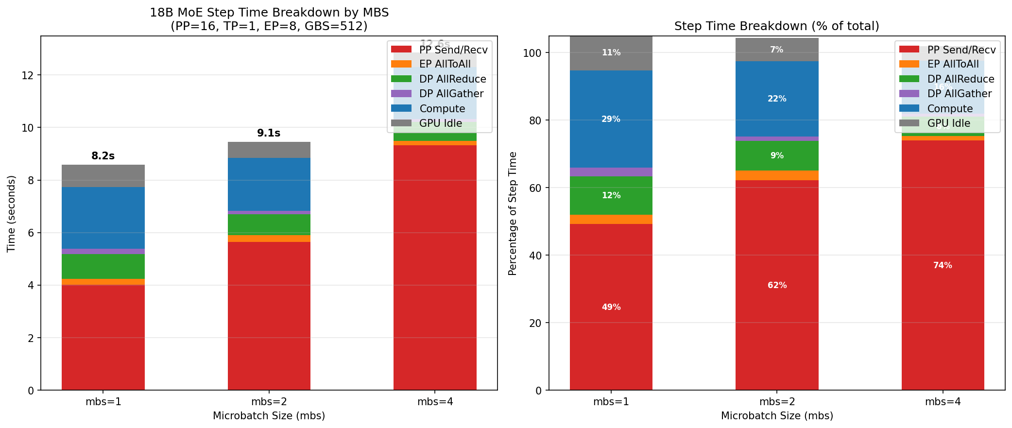
Now $n_{ub} = 512 / (32 \cdot mbs)$ is 16 / 8 / 4 for mbs ∈ {1, 2, 4}.

18B MoE step-time breakdown at GBS=512, PP starvation dominates
At GBS=512 the pipeline is starved. PP communication consumes 49–74% of step time, and mbs=1 wins because it maximizes pipeline fill.

	mbs=1	mbs=2	mbs=4
Step time (s)	8.2	9.1	12.6
PP total (s)	4.0	5.6	9.3
Theoretical bubble $(P - 1) / n_{ub}$	93.8%	187.5%	375%
PP Recv max single call (ms)	261	3,720	7,837

Look at that bubble fraction. With PP=16 and $n_{ub} = 4$ , the formula gives 375% bubble, meaning the pipeline is idle for nearly 4× the useful compute time. There is no 1F1B steady state at all. The entire schedule is warmup followed by cooldown. Rank 0 fires its 4 forwards in ~572 ms, then waits 9.3 s for gradients to come back through 15 stages. The single longest PP Recv is 7.8 s, which is one backward traversal of the full pipe.

The direction reversal is exactly what the iteration-time formula predicts,

T_{iter} \approx \underset{useful}{\underset{⏟}{n_{ub} \cdot t_{ub}}} + \underset{bubble}{\underset{⏟}{(X_{PP} - 1) \cdot t_{ub}}} + \dots

When $n_{ub} ≫ X_{PP}$ , the bubble is a small overhead and you want larger $mbs$ to amortize launch tax and improve $η$ . When $n_{ub} \leq X_{PP}$ , the bubble dominates and you want as many microbatches as possible, so smallest $mbs$ wins.

A rule of thumb follows directly from the formula.

bubble fraction = \frac{X_{PP} - 1}{n_{ub}} ⟹ n_{ub} \geq 2 X_{PP} for bubble \leq 50 %, n_{ub} \geq 4 X_{PP} for \leq 25 % .

For PP=16, you want $n_{ub} \geq 32$ to be in tolerable territory and $n_{ub} \geq 64$ to be comfortable. Below the threshold, the cost model picks a different winner, and the only way to predict that is to carry the pipeline-bubble term explicitly in the model. If you only carry compute and bandwidth, you will recommend mbs=4 in both cases and be wrong by 50% on the second one.

There is also a smaller but instructive pattern in the same profile, where PP Send dominates Recv at GBS=8192 but Recv dominates Send at GBS=512. With many microbatches, rank 0 is backlogged trying to push activations into a busy pipe. With few microbatches, rank 0 finishes pushing immediately and waits for gradients. Same kernel name, opposite physics, and the model captures both as the same $T_{ring}$ rule with different $S$ and $n$ .

11. A Practical Profiling Workflow

The pieces above compose into a workflow that can actually be run.

Predict before you measure. Write down $T_{iter}$ as a sum of the operator costs above, even roughly. You will catch most "huh, that's slow" moments before launching a 512-GPU job.
Decompose the NCCL bucket. Do not trust kernel-name grouping. Use the process-group descriptor (PIPELINE_MODEL_PARALLEL_GROUP, EXPERT_MODEL_PARALLEL_GROUP, DATA_PARALLEL_GROUP) to attribute time to PP / EP / DP. Otherwise PP P2P and EP A2A get conflated under ncclDevKernel_SendRecv.
Compare per-microbatch costs, not per-step. Per-step totals can hide the actual physics. PP per-ub goes 95 → 195 → 445 ms at GBS=8192 (linear in mbs, bandwidth-bound link). EP A2A per-ub goes 14 → 29 → 50 ms (linear in mbs). Compute per-ub is roughly linear too. These linearities are a sanity check. If a per-ub cost grows super-linearly, you are crossing a protocol or load-balance threshold.
Always sanity-check the bubble. $(X_{PP} - 1) / n_{ub}$ takes 5 seconds to compute and instantly tells you whether your schedule is in the "kernel efficiency wins" regime or the "pipeline fill wins" regime.
Distinguish exposed vs overlapped collectives. $T_{DP}^{exp}$ is what hurts you. The naive "DP AllReduce total" in a profile usually undercounts the exposed time because it includes overlap. Subtract the overlap window explicitly.
Do not trust an averaged number when the step has a straggler. A single 8.7s AllReduce in a 65s step can warp every aggregate metric. Always look at P99 / max alongside the mean.
Be explicit about whether your MFU uses active or total parameters. MoE ratios make this a 2–4× lie if you mix it up.

12. Why This Way of Thinking Matters

The honest reason to build a per-operator iteration-time predictor, instead of staying with max(compute, I/O), is that the optimal layout depends on terms the roofline cannot see. Pipeline-bubble curvature, kernel-launch tax, NCCL protocol thresholds, and EP all-to-all inter-node fractions are not second-order terms. At small GBS or deep PP, they choose the winner.

A useful frame is that the roofline tells you which side of the device a kernel is bound on, while the operator-level model tells you which side of the cluster a step is bound on. The first is local to a kernel. The second is what determines training throughput.

The flip side is that when you do this, you are no longer guessing. The 18B / GBS=8192 / mbs=4 result and the 18B / GBS=512 / mbs=1 result are not contradictions. They are what the same iteration-time formula predicts at two different operating points. Once you see that, profiling becomes much less of a "look at flame graph and squint" exercise and much more of a "predict, measure the residual, attribute the residual" loop.

The takeaway from this post is a vocabulary (GEMM rule, HBM rule, ring/A2A rule, bubble term, launch tax, exposed DP comm, AdamW R/W) and a habit of adding terms until the prediction matches the trace, rather than trying to reason from a single roofline. The operator decomposition is more work upfront, but it is the only thing that scales as you start asking questions like "should I switch from PP=16 to PP=8 with TP=2?", questions where every term in $T_{iter}$ moves at once.

References and Further Reading

Williams, Waterman, Patterson, Roofline: An Insightful Visual Performance Model for Multicore Architectures, the original roofline.
Dao et al., FlashAttention, for the SDPA arithmetic-intensity treatment.
Narayanan et al., Efficient Large-Scale Language Model Training on GPU Clusters Using Megatron-LM, for 1F1B and the $(P - 1) / n_{ub}$ bubble.
NVIDIA, NCCL Performance Tuning, for the LL/LL128/Simple protocols and their size thresholds.