Sparse MoE Pretraining with Adaptive Computation

This blog post is a follow-up to my earlier scaling law studies on MoE training. While that post examined how MoE models scale across different dimensions, this work focuses on making MoE models adaptive—enabling them to dynamically adjust computation per token rather than using fixed compute as in traditional conditional computation approaches.

Note: The approaches discussed in this post apply to the traditional non-fine-grained MoE architecture setting, where entire FFN layers are replaced with expert modules (as in Switch Transformers, DeepSpeed MoE, etc.), not fine-grained MoE where individual experts within layers are subsequently partitioned.

Introduction

Not all tokens in a sequence require the same amount of computation (FLOPs in a forward pass). However, the need for adaptive compute for some tokens is not unique to MoE-style models—the training for such could be adjusted for any dense model. Past work on adaptive computation (where FLOPs per token are reduced without reducing total parameter count) in dense models mainly involves early layer exit strategies.

This exploration presents a novel approach to sparse MoE pretraining that combines the benefits of expert specialization with adaptive per-token computation, going beyond the fixed-compute limitations of traditional MoE architectures.

Recap of MoE Setup

You can skip this section if you're already familiar with conventional MoE setups like Switch Transformers.

MoE Architecture
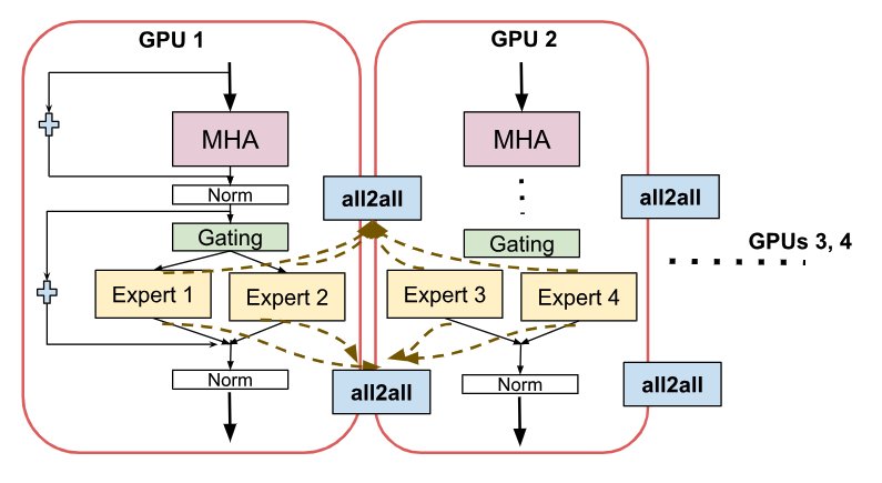
Figure 1: GPT-2 decoder with MoE layers replacing FFN in alternate transformer blocks

We follow a GPT-2 decoder architecture where the FFN in every alternate transformer layer block is replaced by the MoE layer having multiple copies of the FFN layer as expert modules.

Key MoE Characteristics

Sparse Routing: Typically, 1 or 2 experts per token are selected per MoE layer in a forward pass through a router
Sparse Backpropagation: Gradients only flow through the selected experts for each token
Expert Parallelism: The distributed nature of expert placement across GPUs is crucial—communication becomes a bottleneck and is instrumental in deciding the architecture and routing strategy
Top-1 Preference: 1 expert per token is always desirable for communication efficiency, although it may not be the optimal choice for model quality

Routing Mechanism

We follow the Switch Transformer style greedy routing/gating function:

Router parameterized by $W \in R^{d \times M}$ for $M$ experts
Produces logits based on preceding multi-head attention output
Logits normalized via softmax distribution over available experts
Top-k token-choice: Select top-k experts per token based on normalized router probabilities

Load Balancing

An auxiliary differentiable load balancing loss is introduced:

loss = α \sum_{i = 1}^{M} f_{i} \cdot P_{i}

where $f_{i}$ represents the fraction of tokens dispatched to expert $i$ , and $P_{i}$ is the fraction of the router probability allocated for expert $i$ .

What Are We Trying to Improve?

The Capacity Factor Problem

In MoEs, the capacity factor of an expert (a hyperparameter controlling the maximum number of tokens each expert in one MoE layer is allowed to process in a batch) determines the FLOPs upper bound of a sequence in a routed MoE model—not just the total sequence length and not the outcome of the routing decision.

Capacity Factor Impact
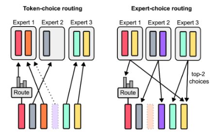
Figure 2: How capacity factor determines compute bounds in MoE layers

Advantages of MoE for Adaptive Compute

MoE models have some implicit advantages for adaptive computation since we already have the router as a decision maker. This proposal differs from plug-and-play approaches to language model compositions—this is a parallel exploration where "layers" are tied and routed to instead of entire models being routed.

Existing Methods for Adaptive Compute in MoEs

Weight Tying (Universal Transformers/ACT)

These techniques are similar to vertical exits where compute is reduced through weight sharing across layers. They are mainly effective for algorithmic tasks like mathematical calculations.

Advantages: In algorithmic tasks like parsing nested mathematical expressions or programming code, applying the same logical rules at every depth of input processing can improve generalization.

Disadvantages:

Unfortunately, ACT is notably unstable and sensitive to hyperparameter choices
The gradient for the cost of computation can only backpropagate through the last computational step, leading to biased gradient estimation
Universal Transformers are very restricted to certain tasks

Dynamic Top-k for Each Token

Instead of selecting the same k in top-k per token, select different k based on some criteria.

Bottlenecks:

If using a threshold-based method, introduces a new hyperparameter that either needs calibration during training or requires a calibration layer for softmax probabilities
When k is large for some tokens, this introduces significant communication overhead with expert parallelism

Expert Choice Routing

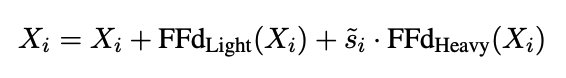
Figure 3: Expert choice routing where experts select tokens

Expert choice routing performs softmax expert selection from an expert perspective, allowing a dynamic number of experts per token.

Disadvantages:

Expert selection for a token is non-causal, requiring an auxiliary router for autoregressive decoding
To cap number of experts per token, need constraints and IP formulation
More experts per token still has communication issues

Mixture of Depths (MoD) and ColT5

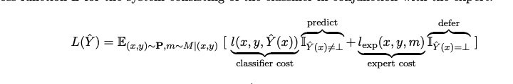
Figure 4: Mixture of Depths allowing tokens to skip layers

MoD is similar to early exit techniques where the router decides which tokens in a sequence will skip an MoE layer.

Characteristics:

Uses expert choice routing where probabilities for a token are ordered
Uses a threshold hyperparameter deciding what percentile of tokens in a batch will skip the MoE layer
No latency benefit in pretraining as you still wait for other tokens in a batch for loss computation

ColT5 is similar but uses routing to decide whether to "add" more compute instead of cutting compute—our proposed method is similar in nature.

Proposed Approach: Heterogeneous Experts

Core Concept

One way of allowing dynamic compute is to partition the FFN layer in an MoE such that we can jointly optimize the splits and choose 1 expert/partition per token. But achieving this in pretraining at scale is expensive, so we start with a simpler case.

Heterogeneous Experts
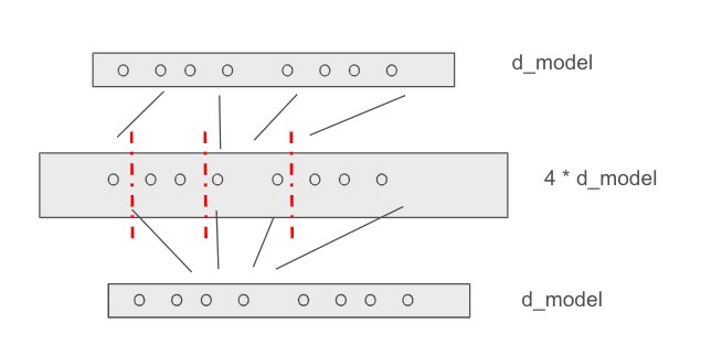
Figure 5: Partitioning experts into different sizes for adaptive computation

Expert Partitioning Strategy

Consider the uniform expert case where for a given MoE layer with K experts each having hidden dimension $d_{f f}$ , the total hidden size is $K \cdot d_{f f}$ .

Goal: Split the hidden dimension $K \cdot d_{f f}$ into K partitions/experts such that we have non-uniform experts, where some experts are larger than others with respect to hidden dimension.

Initial Setup: Split the FFN network into K experts such that:

K-1 experts have the same P parameters each
One expert has xP parameters, where x is a predetermined hyperparameter (not learned)
We call the larger expert $m_{a c c}$

Pretraining Desiderata

Expert Specialization: Want smaller experts to be specialized as in traditional sparse MoE models with learned routing
ERM Perspective: Loss incurred from routing with the larger expert should be no worse than the smaller expert (though this may not strictly hold due to expert specialization)
Compute Bounds: Compute per sequence is upper bounded (horizontally/vertically) as with uniform routing—ensures reducing compute for some tokens can be adjusted by adding compute for other tokens in a sequence
Uniform Utilization: Globally, smaller experts are more uniformly utilized as in top-2 case (unlike top-1)

Inference Desiderata

Causality: 1 expert per token with causal nature of expert selection
Latency: Inference latencies are no worse than top-1 routing and better than top-2 routing

Key Challenge

The main challenge is handling the dichotomy between:

Expert specialization with learned routing (more experts given a FLOP budget is always better)
Hardness-based adaptive compute with heterogeneous experts requiring explicit routing signals

The latter impacts expert specialization, so the problem is achieving the best of both with heterogeneous experts.

Routing Algorithm

There are two main problems to solve:

Bounding compute per batch/sequence: Amount of compute should not exceed the uniform expert case
Token-to-expert assignment: How to decide which tokens to allocate more compute during routing

Two Routing Paradigms

Experts choose tokens:

Assignment is prioritized for experts
Algorithms like ECR and EPR let experts choose tokens
Easy to balance expert usage explicitly
⚠️ Non-causal routing - major blocker for autoregressive decoding

Tokens choose experts:

Tokens decide scores for experts independently
Balancing cannot be achieved implicitly; done through regularization
✅ Causal routing - can be directly used in autoregressive decoding

Our Approach: Hybrid Routing

We perform routing both at sequence and batch levels:

Batch level: Can be non-causal (among sequences)
Sequence level: Must be causal

Batch and Sequence Setup

Let a batch consist of N sequences of tokens. Each sequence $S_{i}$ contains $P_{i}$ tokens, so the batch has a total of $\sum_{i = 1}^{N} P_{i}$ tokens.

Capacity Constraints: Each expert has finite capacity. Let $C$ be the total capacity for the batch, where $C = 1$ . The goal is to distribute this capacity among sequences while ensuring total batch capacity equals 1.

Non-Causal Batch-Level Capacity Allocation

Sequence-Level Priority Score: For each sequence $S_{i}$ , compute a sequence-level priority score based on token difficulty:

s (S_{i}) = \sum_{t = 1}^{P_{i}} difficulty (x_{t})

Capacity Allocation per Sequence: Allocate a fraction of the batch's total capacity based on priority score:

C_{i} = \frac{s (S_{i})}{\sum_{j = 1}^{N} s (S_{j})}

This ensures sequences with higher priority scores (more difficult tokens) receive a larger share of capacity.

⚠️ Non-causal: This allocation depends on difficulty scores of all tokens across all sequences in the batch.

Causal Token-Level Routing

Once capacity is allocated to each sequence, apply causal token-level routing within each sequence.

Dynamic Batch Construction

We will explore designing batch construction such that each batch consists of sequences with similar token difficulties, ensuring smoother capacity allocation. This can involve dynamically adjusting sequences included in each batch based on their difficulty scores.

Inference Implications

Inference Strategy
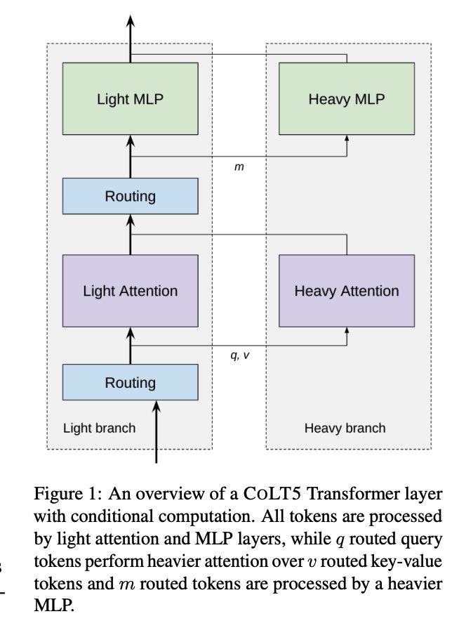
Figure 6: Inference phase strategies for prefill and decoding

Any production deployment is considered viable if:

Our compute-bounded training results in better performance than top-2 uniform experts
Our inference throughput is better or close to top-2 uniform

Prefill Phase

In the prefill phase where the entire prompt sequence is processed in parallel, we can avoid bottlenecks for batch decoding by utilizing only the smaller experts. Since all tokens are processed simultaneously, using only smaller uniform experts prevents delays from slower larger experts.

Decoding Phase

We modulate the performance vs inference tradeoff through a threshold hyperparameter knob:

Single Sequence (Batch Size = 1):

Fall back to normal decoding where threshold is for token difficulty score
Decides whether to use larger expert
Some calibration needed to ensure larger experts are used less on average
No additional bottleneck: Overhead from larger experts for some tokens compensated by faster inference from smaller experts for others (similar to CALM)

Batch Decoding:

Bottleneck arises when for a single position, a sequence using the larger expert causes delay
Mitigation: Use non-causal expert-to-token selection where larger experts select top-S tokens based on difficulty scores

Open Research Problem

An interesting research problem is how the notion of easy and difficult tokens based on rejection sampling (as in speculative decoding) can be utilized in the pretraining stage to decide routing. This could make routing decisions in pretraining and inference closer.

Training Algorithm

Training Algorithm
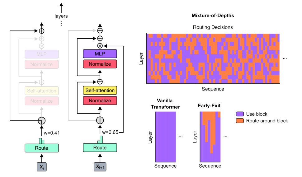
Figure 7: Two-stage training approach for heterogeneous MoE

We follow a 2-stage approach to train MoE layers with heterogeneous experts.

Stage 1: Training Experts Without Routing

Initialization:

Initialize all experts
Learn two sets of weights for each MoE layer:
- Weights of the larger expert $m_{a c c}$
- Weight of one small expert (used to initialize K-1 smaller experts with perturbation)

Training:

Train these two experts on tokens using round-robin gating
May need gradient scaling or batch-wise balancing so larger expert receives more tokens
This stage consumes a significant portion of total compute

Note: EvoMoE does a similar kind of routing with two stages.

Stage 2: Router Learns to Assign Tokens to Experts

For each token in a batch:

Compute router probabilities among all experts
Pick top-1 among smaller experts
Compute loss $L_{s}$ for forward pass with selected smaller expert
Compute $L_{a c c}$ for forward pass with larger expert

Goal: Route harder-to-predict tokens through appropriate experts. A hard example is one where larger experts can classify better than smaller ones.

Router Loss

We use a router loss:

L_{router} = - \frac{1}{N} \sum (y_{i} \log (p_{i}) + (1 - y_{i}) \log (1 - p_{i}))

where:

y_{i} = σ (τ \frac{L_{s} - L_{a c c}}{L_{s}})

and $p_{i}$ is the probability of selecting the larger expert.

Interpretation:

If $L_{s} > L_{a c c}$ : $y_{i}$ closer to 1, indicating larger expert performed better
If $L_{s} < L_{a c c}$ : $y_{i}$ closer to 0, indicating smaller expert performed better

Local Proxy Loss

The bottleneck is that the loss gap $y_{i}$ needs to be computed such that other MoE layers don't contribute their errors into this gap. We employ a local MoE layer-specific proxy loss that approximates $L_{s}$ and $L_{a c c}$ .

Steps:

Given input $x$ , router $R (x)$ outputs logits $l = [l_{1}, \dots, l_{K - 1}, l_{a c c}]$
Compute probabilities for experts using softmax top-k routing
Compute local losses $L_{L} = L (E_{a c c} (x))$ and $L_{S_{i}} = L (E_{S_{i}} (x))$ for selected smaller expert
Add router loss to cross-entropy loss (introduces new hyperparameter)
Add usual load balancing auxiliary loss ensuring tokens are equally distributed to smaller experts

Modulating Capacity per Sequence

To ensure the larger expert is not utilized more often than smaller experts in a sequence and throughput is not bottlenecked:

Add regularization term that minimizes the difference between:

Capacity utilized if all tokens used smaller experts
Actual allocation that happens

Baselines

For comparison, we implement existing low-cost methods that allow varying compute per token or sequence during inference:

K1: Expert Choice Routing with Auxiliary Router

Copy the existing auxiliary router method proposed in MoD for autoregressive decoding. Introduces a small auxiliary MLP predictor (akin to a second router) that receives the same inputs as the router (with stop gradient), whose output is a prediction whether that token will be among the top-k in the sequence.

Does not affect language modeling objective
Empirically does not significantly impact step speed

K2: Adaptive k in Top-k During Inference

Goal: Pretrain the router to be robust to adaptive k during inference (per-token, per-sequence, or per-task).

Current Empirical Observations:

For few expert cases (16 and 32): Using top-1 for eval with top-2 pretrained checkpoint degrades performance totally
For 128 expert case (smaller experts): Using top-1 for eval with top-2 pretrained checkpoint does not degrade performance significantly
Conclusion: For larger experts and fewer of them, adaptive compute is sensitive and algorithmic accommodation in pretraining is necessary

Mitigation Approaches:

Multi-k Pretraining: Allocate some tokens or sequences higher k in top-k for flexibility during inference
Soft Gumbel-Softmax Noisy Routing: Apply Gumbel-Softmax noise trick to allow soft expert selections. Anneal temperature during training to make selection more discrete
Straight-Through Gumbel-Max Estimator: Use hard argmax selection during training to improve generalization when changing k. Addresses the issue where softmax weights blur expert selection

Follow-Up Questions

1. Allocating Adaptive Compute per Sequence

The current method doesn't ensure that on a per-sequence basis, total FLOPs remain similar to the uniform top-1 expert case. May need to add regularization to penalize too-frequent routing to the larger expert.

2. Generalizing to All Heterogeneous Experts

We can make all experts non-uniform in their sizes, although we need to understand why that would be advantageous in terms of expert specialization.

3. Expert Parallelism Dispatch Masks

Do we need different dispatch masks for expert parallelism to handle heterogeneity? Yes, but for initial experiments with smaller MoE models (300-600M parameters), we hope not to modify EP.

4. Adaptive Compute in Self-Attention

Should we also handle adaptive compute in self-attention? This is complementary and can be incrementally added later.

5. Alternative Learning Methods

Are there other parallel methods for learning how to defer to larger experts? Cost-sensitive learning loss functions could be explored.

Alternative Approaches

Gradient Norm-Based Routing

An alternative to loss difference could be measuring gradient norm using the local loss function:

For each token $x$ passing through an MoE layer, compute local proxy loss $L_{local}$ during forward pass. Approximate gradient norm using first-order approximation:

∥ \nabla_{x_{t}} L_{local} (x_{t}) ∥ \approx | \frac{\partial L_{local}}{\partial h (x_{t})} | \cdot | W_{local} |

where $h (x_{t})$ is the hidden state output, and $W_{local}$ are the layer weights.

Routing Decision:

High gradient norm → route to larger expert
Low gradient norm → route to smaller expert

⚠️ Major Issue: These measures cannot be used in inference as there is no gradient during decoding.

Key Insights and Contributions

Heterogeneous Expert Architecture: First systematic exploration of non-uniform expert sizes in sparse MoE models for adaptive computation
Two-Level Routing: Novel approach combining non-causal batch-level capacity allocation with causal token-level routing
Training Stability: Two-stage training approach that first establishes expert capabilities before introducing routing
Inference Flexibility: Different strategies for prefill (uniform small experts) vs decoding (adaptive expert selection) phases
Production Viability: Design considers both model quality and inference throughput constraints
Empirical Insights: Observation that smaller, more numerous experts are more robust to adaptive k during inference

Conclusion

This work presents a comprehensive framework for incorporating adaptive computation into sparse MoE models during both pretraining and inference. By introducing heterogeneous expert sizes and sophisticated routing mechanisms, we can potentially achieve:

Better compute efficiency through per-token adaptation
Improved model quality through better expert specialization
Practical deployment with inference-time flexibility

The key innovation lies in recognizing that MoE models, with their inherent routing mechanisms, are naturally suited for adaptive computation—we just need the right architectural and algorithmic components to unlock this potential.

Future work will focus on:

Empirical validation of the proposed methods
Scaling to larger model sizes and expert counts
Integration with other efficiency techniques like speculative decoding
Exploration of fully heterogeneous expert architectures

This represents a step toward truly adaptive neural networks that can dynamically allocate computation based on input complexity, moving beyond the fixed-compute paradigm of traditional neural architectures.

References

Switch Transformers: https://arxiv.org/abs/2101.03961
Mixture of Depths: https://arxiv.org/abs/2404.02258
Expert Choice Routing: https://arxiv.org/abs/2202.09368
ColT5: https://arxiv.org/abs/2303.09752
CALM: https://arxiv.org/abs/2207.07061
EvoMoE: https://arxiv.org/abs/2112.14397
Cost-Sensitive Learning: https://arxiv.org/pdf/2006.01862
Gumbel-Softmax: https://arxiv.org/abs/2002.07106
Plug-and-Play Language Models: https://arxiv.org/pdf/1912.02164