Scaling Law Studies on Mixture of Experts Training

Note: This blog post was written in late 2023 and some findings may be outdated given the rapid developments in MoE architectures since. However, I kept this up since it provides valuable insights into the scaling aspects of mixture of experts models that remain relevant for understanding the fundamentals of sparse model training.

Introduction

Scaling language models with more data, compute and parameters has driven significant progress in natural language processing. Now that studies have shown Mixture of Experts (MoE) can lead to better performance when scaled from their respective dense models and when they are compute FLOP matched per token, the key observations we need to aggregate and the follow up questions we need to answer for our own work are the following:

• What are the dimensions of scaling to keep in mind when adding MoE layers in dense models and what laws have been observed so far w.r.t. those dimensions when comparing training/validation losses and downstream task performances?
• When considering the dense models, do we see the same improvements with MoE on smaller dense models as we do with larger dense models i.e. given improvements on one of the dimensions w.r.t. training cost (loss over steps or loss over token count) with a dense model of size M parameters, do we see the same improvements with similar scaling starting with dense models of size much larger like 5M?
• Do we see the same improvements as we do with training/validation loss on downstream task performance?

The goal of answering the above three questions is to decide on how to scale our own dense models if we were to start from pretrained checkpoints of dense models and not pretrain from scratch.

Models Considered

The following models from related papers are considered in the comparisons:

Switch Transformers (Fedus et al. 2022)

Base dense models are T5 encoder-decoder models. In Switch, the routing follows top-1 i.e. each token is routed to only 1 expert per MoE layer. The load balancing is performed using an auxiliary loss and the MoE layers replace every other FFN layers in the transformer component. Families of models are trained varying by the number of experts in each layer and the dense models parameter count.

ST-MoE (Zoph et al.)

This model is an improvement over the Switch transformer with added router losses to improve training stability (remove loss divergences) and scale a sparse model to maximum 269B parameters, with a computational cost comparable to a 32B dense encoder-decoder Transformer. The sparse models are FLOP matched to T5-XL (3B). An MoE layer is introduced for every fourth FFN.

Small models are rarely unstable but large unstable models are too costly to run for sufficient steps and seeds. They found a sparse model FLOP-matched to T5-XL to be good object of study because it was unstable roughly 1/3 of the runs, but was still relatively cheap to train.

DeepSpeed MoE (Rajbhandari et al.)

Studies GPT-like transformer-based NLG model (decoder only autoregressive). The following models are selected:

• 350M: 24 layers, 1024 hidden size, 16 attention heads
• 1.3B: 24 layers, 2048 hidden size, 16 attention heads
• 6.7B: 32 layers, 4096 hidden size, 32 attention heads

The notation "350M+MoE-128" denotes a MoE model that uses 350M dense model as the base model and adds 128 experts on every other feedforward layer. That is to say, there are in total 12 MoE layers for both 350M+MoE-128 and 1.3B+MoE-128. Only the top-1 expert is selected.

GLAM (Du et al.)

Proposes and develops a family of language models named GLaM (Generalist Language Model), which uses a sparsely activated mixture-of-experts architecture to scale the model capacity while also incurring substantially less training cost compared to dense variants. The largest max base dense model is 64B parameters scaled to 1.2T parameters and FLOP/token matched to 96B. Uses top-2 routing.

Unified Scaling Laws for Routed Language Model (Clark et al.)

In this work, three models are considered:

• S-Base (Sinkhorn base): Base model where the token to expert (top-1 match) is done using Sinkhorn matching instead of Hungarian matching
• Hash layer model (HASH): Tokens in this model are routed to fixed experts based on their hash
• RL based routing model (RL-R): Each router is seen as a policy whose actions are the selection of an expert in each routed layer and whose observations are the activations passed to that router. After completing the forward pass, the probability the Routed Transformer assigns to the correct output token can be used as a reward, maximization of which is equivalent to minimization of NLL.

Key Observations

Summarizing the findings from the studies, I found the following:

• All scaling studies done on sparse MoEs have been done with smaller dense models (mostly < 20B). The GLAM paper is the only one that scales a 64B dense model to 1.2T parameters. The Switch transformer also scales a model between 3B and 11B params to a 1.5T param model by introducing 2048 expert layers. In both of these, the results are better when considering validation perplexity compared to their FLOP matched dense models. So questions remain on what would happen with larger dense models like 200B when scaled to trillion params.

• It is clear that for smaller dense models (<2B), using routing even with top-1 routing and scaling them to 4-5x sparse model params results in better models. The main reasons behind low adoption is the communication overhead, instability and the added load balancing loss which creates maintainability issues.

• GLAM model shows that scaling a 64B model to 1.2T with 1.6T tokens improves the results while the Unified Scaling Laws for Routed Language Model (Clark et al.) hypothesizes with some data fit that routing would not help with larger models beyond a cutoff size. However, that hypothesis is not clear as the analytic functions used to derive this conclusion were fit only on data from smaller dense models scaled to sparse MoEs.

There are several dimensions along which scaling has been measured for models with routing based sparsity. These dimensions are:

• Number of experts
• Expert capacity
• The dense (base) model size
• The effective parameter count (which is the FLOPs/token matched equivalent dense model)

Scaling Results on a Step/Tokens Basis

Switch Transformer (Encoder-Decoder Model)

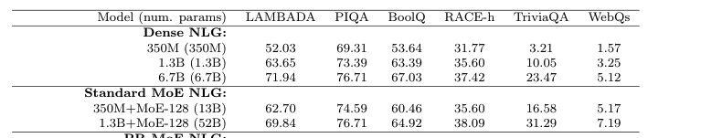
Figure 1: Switch Transformers MoE models with different number of experts added to the T5-base model

The above plot with Switch Transformers shows that the MoE models with different number of experts added to the T5-base model. Results show that when the FLOPs/token are constant, increasing the experts for a T5 base (770M) model results in better negative log perplexity (higher is better) over the training steps.

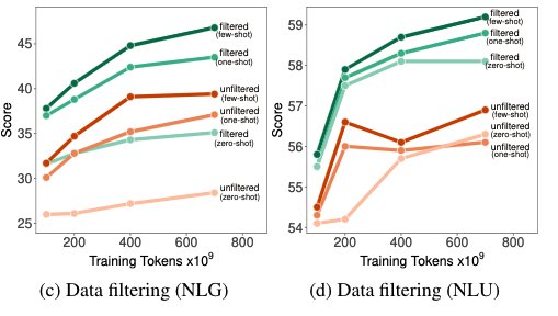
Figure 2: Speedup considering wall clock time to reach target perplexity values

This plot shows the speedup considering the wall clock time taken to reach values of log perplexity. The 64 expert Switch-Base model achieves the same quality in one-seventh the time of the T5-Base. Note that all these models are compute FLOP matched per token since this is top-1 routing.

DeepSpeed MoE

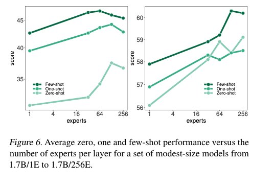
Figure 3: DeepSpeed MoE validation loss comparison

When comparing the losses over the tokens, the DeepSpeed MoE work showed that "350M+MoE-128 is on par with the validation loss of the 1.3B dense model with 4x larger base". One thing to note that the 350M+MoE-128 has a total of 13B parameters but compute FLOP/token matched to 350M.

This conclusion in my opinion is very positive. It tells us that by just splitting the FFN into multiple networks and even though the individual expert networks have seen fewer tokens in training compared to the dense model after certain tokens, it still performs equal to a much larger dense model. So a first experiment in scaling could just be this: split the FFN networks with top-1 routing and see the results.

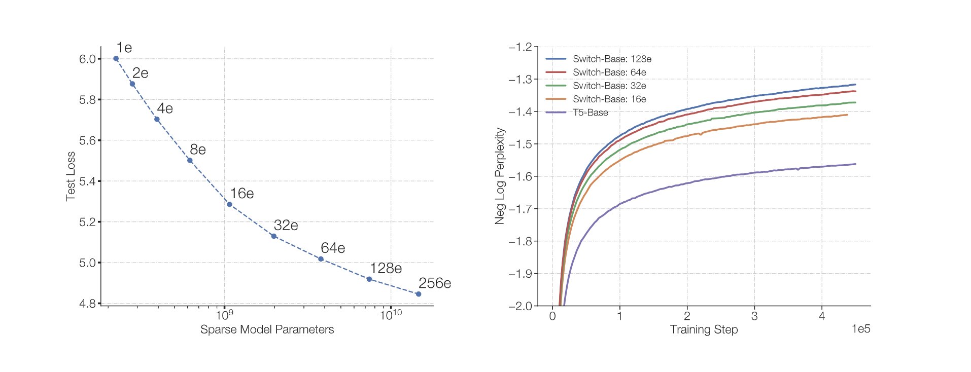
Figure 4: DeepSpeed MoE results on downstream tasks

Note that these results also transfer to downstream tasks:

• 350M+MoE-128 is on par with the validation loss of the 1.3B dense model with 4x larger base
• This is also true for 1.3B+MoE-128 in comparison with 6.7B dense model with 5x larger base

GLAM

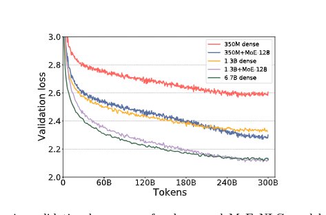
Figure 5: GLAM MoE models vs dense counterparts

The results of GLAM MoE models show that the MoE models and their dense counterpart with 4-5x larger base have very similar model quality. This is the same conclusion as the one with DeepSpeed-MoE.

64B/64E means that the base dense model is 64B decoder with 64 expert scaling. GLaM MoE models perform consistently better than GLaM dense models for similar effective FLOPs per token.

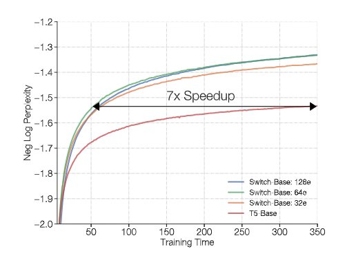
Figure 6: GLAM MoE data efficiency comparison

GLaM MoE models require significantly less data than dense models of comparable FLOPs to achieve similar zero, one, and few-shot performance. In other words, when the same amount of data is used for training, MoE models perform much better, and the difference in performance becomes larger when training up to 630B.

Scaling Results with Number of Experts

Switch transformer work mentions that number of experts is the most effective dimension for scaling in MoE models.

The number of experts is the most efficient dimension for scaling our model. Increasing the experts keeps the computational cost approximately fixed since the model only selects one expert per token, regardless of the number of experts to choose from. The router must compute a probability distribution over more experts, however, this is a lightweight computation of cost $O(d_{\text{model}}\times \text{num\_experts})$where $d_{\text{model}}$is the embedding dimension of tokens passed between the layers.

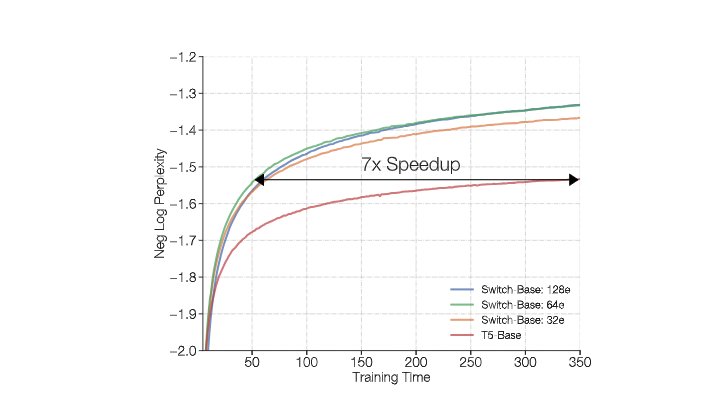
Figure 7: Switch Transformer scaling with number of experts

For the Switch transformer results, it is clear that increasing the number of experts improves the results compared to the dense model although it seems to saturate comparing 64 and 128 experts which the paper does not seem to highlight. So it could be that for smaller models as these, there is a threshold after which there are diminishing returns with increasing number of experts.

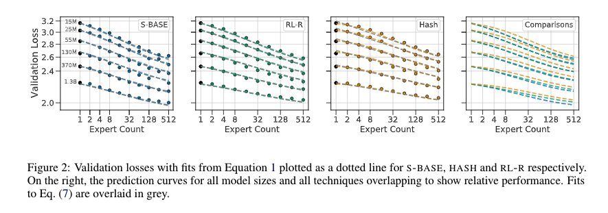
Figure 8: Unified Scaling Laws showing loss vs number of experts

The Unified Scaling Laws paper shows above that with increasing experts the losses decrease almost linearly with increasing experts till 512. The dense model sizes for each curve is in the plot. All these use top-1 routing. The results show that the Base model method (which used the Hungarian matching) to assign 1 expert to each token is pretty effective and surpasses costly RL based or hash based methods.

Figure 9: GLAM decoder model expert scaling results

The results for the GLAM decoder only GPT style model shows that for the 1.7B models, increasing the number of experts improves the results. Even with these results, it is not clear whether there is a threshold after which the number of experts do not scale.

There are some other factors like expert capacity (which is number of tokens/number of experts × capacity factor), the capacity factor, the Top-K factor and the top-k MoE layer interval which also impact the results but they are mostly dependent parameters themselves. For example, it was conjectured that MoEs require (K>2)-way routing to produce effective gradients in the routers, and many attempts at incorporating routing into large Transformers use K=2. However recently this has been challenged, and stable modifications have been proposed for K=1; namely the Switch Transformer. Most MoEs, including Switch, are reliant on auxiliary balancing losses which encourage the router output to be more uniform across mini-batches of inputs.

Scaling Issues with Out-of-Distribution Data

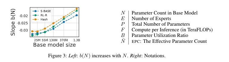
Figure 10: In-domain vs out-of-distribution performance

The paper observes these when comparing dense vs sparse MoEs on in vs out-of-distribution validation measures:

• All MoE models outperform their dense counterparts in all datasets, but their advantage greatly varies across domains and models
• MoEs are most efficient when evaluated in-domain, where they are able to match the performance of dense models trained with 8-16x more compute
• The improvement is more modest in out-of-domain settings, bringing a speedup of 2-4 on the Pile. This is reflected in the figure above where the gap between the MoE and dense curves is substantially smaller in out-of-domain settings

How to Scale MoE Models

The main question is then how do we scale the models. From the observations above, the results are clear for smaller dense models (< 60B) and it also seems that for each model there is a threshold number of experts beyond which there are diminishing returns. At the same time, just using top-1 routing and scaling to few experts should still improve the results. So what is the catch then in using these models? In my opinion, it is mainly the routing and the instabilities that come along with it.

Before going into some analytical observations from Unified Scaling Laws for Routed Language Model (Clark et al.), these are the common configurations of expert models:

GShard (Lepikhin et al.)

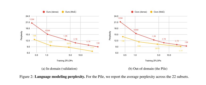
Figure 11: GShard MoE configuration

DeepSpeed MoE Configuration

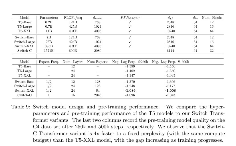
Figure 12: DeepSpeed MoE architecture configuration

Switch Transformers Configuration

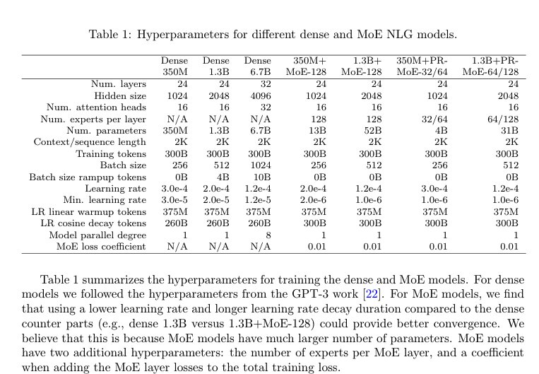
Figure 13: Switch Transformer configuration details

Analytical Scaling Laws

The paper Unified Scaling Laws for Routed Language Model (Clark et al.) posits that the loss dependent on number of experts can be written as follows for top-1 routing:

where $N$denotes the parameter count of the base dense model.

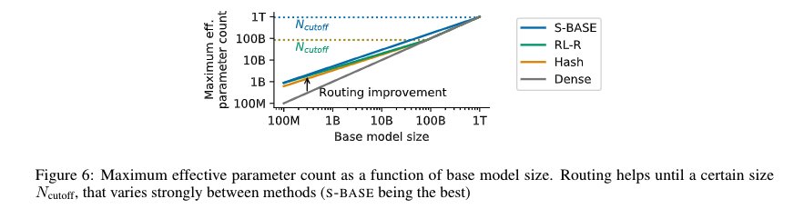
Figure 14: Plot showing slope b dependent on N

The paper goes on to give an analytic function to decide the effective parameter equivalence. To compute the effective parameter count that gives the same performance as the sparse MoE, $N$denotes the effective parameter count, $N$denotes the base dense model size:

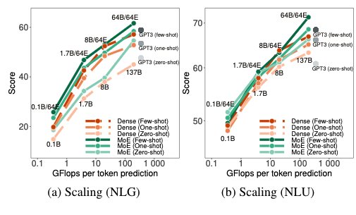
Figure 15: Effective parameter count analysis

Figure 16: Analysis of routing effectiveness across model sizes

The discussions on whether there is a cutoff model size beyond which the routing would not help is not clear, since this paper mentions that beyond a certain size, the routing would not help by increasing the effective parameter count starting with a given dense model (figure above). But this conclusion conflicts with the results of GLAM model which showed improvements with 64B model.

Conclusions

The scaling law studies on MoE training reveal several important insights:

1. MoE models consistently outperform FLOP-matched dense models across different architectures (Switch, DeepSpeed, GLAM)
2. Number of experts is the most efficient scaling dimension, though there may be diminishing returns beyond a certain threshold
3. Smaller dense models (<20B) show clear benefits from MoE scaling, but results for very large models (>100B) remain limited
4. MoE models are most effective on in-domain data, with more modest improvements on out-of-distribution tasks
5. Top-1 routing appears sufficient for achieving strong performance while maintaining computational efficiency

The main challenges remain around training stability, communication overhead, and the complexity of load balancing mechanisms. Future work should focus on scaling studies with larger base models and improved routing mechanisms.