Origins and Design of Neural Scaling Laws

This doc is a hybrid between knowledge gathering (not exhaustive) and the things you keep in your head when building a scaling analysis for a new model family, modality, or data mixture.

The introduction recaps the Kaplan → Chinchilla formulations and why those particular functional forms show up so often.
Then I go "backwards from the data" and the architecture: what questions you should ask, what plots to make, and what failure modes tell you the functional form is wrong.
I mostly ignore the "training dynamics knobs" (batch size, LR schedule, optimizer) except where recent work shows they directly bias scaling fits or compute-optimal conclusions.

Introduction and Notation

The Kaplan-Era Baseline

The 2020 OpenAI scaling paper (often referred to as "Kaplan scaling laws") observed that validation cross-entropy (or log-perplexity) follows clean power laws in (i) model size (parameter count), (ii) dataset size / training tokens, and (iii) training compute — provided the other factors aren't bottlenecking you. It also emphasized that many architectural "shape" details (depth vs width, head count, etc.) matter surprisingly little for upstream LM loss within a reasonable range.

A technical detail that became important later: they define model size using non-embedding parameters because it makes the trend cleaner across depths.

The Kaplan parameterization for the loss function is:

L (N, D) = {[{(\frac{N_{c}}{N})}^{α_{N} / α_{D}} + \frac{D_{c}}{D}]}^{α_{D}}

This form is chosen based on three structural principles: (1) it allows rescaling for vocabulary/tokenization changes; (2) as $N \to \infty$ with $D$ fixed, it approaches $L (D)$ , and vice versa; (3) it is analytic at $D = \infty$ with a series expansion in $1 / D$ .

The Chinchilla Form People Actually Fit Today

The 2022 compute-optimal paper ("Chinchilla") formalizes the now-standard additive parametric scaling ansatz for LM loss:

\hat{L} (N, D) ≜ E + \frac{A}{N^{α}} + \frac{B}{D^{β}}

where $N$ is parameter count, $D$ is the number of training tokens seen, and $E$ is the best achievable loss on that data distribution.

Conceptually, the paper motivates this via a classical "risk decomposition" story:

$E$ : "ideal generative process" term, interpreted as a tokenization- and distribution-dependent entropy-like baseline for natural text.
$A / N^{α}$ : "capacity / approximation" term — even if you could train perfectly, finite $N$ underperforms the ideal predictor.
$B / D^{β}$ : "finite data / finite training" term — training on a finite number of tokens leaves reducible loss on the table.

Two important LLM-era clarifications:

In LLM training practice, $D$ is almost always tokens processed (with sampling, mixture reweighting, and sometimes repetition), not "unique documents" or "one epoch".
If you do care about "unique data vs repeated data," you usually need an additional variable (e.g. repetition factor / epochs / "data density") because the same $D$ can correspond to very different novelty.

Compute Constraint and the Compute-Optimal Frontier

Both the Kaplan-era and Chinchilla-era derivations rely on a compute constraint of the form

C \approx k N D

for dense Transformers, where $k$ is an architecture-and-implementation dependent constant.

If you minimize

E + \frac{A}{N^{α}} + \frac{B}{D^{β}}

under $C = k N D$ , the clean closed-form compute-optimal scaling is:

N^{*} (C) \propto C^{β / (α + β)}, D^{*} (C) \propto C^{α / (α + β)}, L^{*} (C) - E \propto C^{- α β / (α + β)} .

The important structure here is: the frontier is where you "balance" the model-limited and data-limited terms.

Also, the statement "power laws are observed only along the compute-optimal frontier" is slightly too strong. What is true is that a single power law in compute $L (C)$ is cleanest along compute-optimal allocations, because off-frontier you can get curvature / plateaus / regime changes. But power-law behavior in $N$ (with sufficient data) or in $D$ (with sufficient capacity) is empirically observed as well.

Reconciling Kaplan vs Chinchilla: Why the Coefficients "Moved"

The two papers reach very different conclusions on compute-optimal scaling:

Kaplan: N_{∖ E}^{*} \propto C_{∖ E}^{0.73}, Chinchilla: N_{T}^{*} \propto C_{T}^{0.50}

A later line of work argues the Kaplan–Chinchilla discrepancy comes from a mix of:

parameter counting conventions,
limited scale coverage,
training protocol choices like warmup and schedule,
and optimizer / batch-size tuning.

So the "why" is not a single knob. It is a bundle of measurement choices and training choices, which is exactly the kind of non-universality people forget when they say "scaling laws are universal."

What Actually Justifies the Chinchilla Loss Form

Empirical Regularity Came First

Power-law learning curves predate modern LLMs. Earlier empirical work across translation, language modeling, image, and speech tasks already showed that performance often follows predictable power laws, though the exponents vary by task and domain.

The Kaplan-era paper then made the LLM-scale case: clean power laws across orders of magnitude, some apparent universality, and the idea that these laws are useful precisely because they allow extrapolation and compute allocation.

The Classical Generalization Story Is the Seed of the Functional Form

In classical learning theory, it is common to decompose expected risk into an approximation term (capacity-limited) and an estimation term (finite-sample). In finite-dimensional settings, the estimation error scaling often takes forms like $O (n^{- 1 / 2})$ or $O (n^{- 1})$ .

The Rahimi-style random feature / kernel line of work belongs to this tradition. With $m$ random features and $K$ samples, you get explicit generalization bounds of the form:

R [\hat{f}] - min_{f \in F_{p}} R [f] \leq O ((\frac{1}{\sqrt{m}} + \frac{1}{\sqrt{K}}) L C \sqrt{\log \frac{1}{δ}})

The mismatch with deep nets is obvious: the exponents empirically are often not locked to $1 / 2$ or $1$ , and they remain stable across huge scale ranges where classical asymptotics are unclear. That is why the community treats the Chinchilla form as a structured empirical ansatz rather than a theorem.

Why "Power Law + Constant" Is Natural in Cross-Entropy

In autoregressive modeling, cross-entropy has a clean information-theoretic interpretation as an entropy term plus a KL divergence from the true distribution to the model distribution.

A complementary way to say the same thing is: language modeling is compression. The compression viewpoint connects prediction loss, codelength, and scaling phenomena, and it is also a practical lens for reasoning about tokenization, modalities, and why "loss floors" are distribution-dependent.

Theory Attempts: Variance-Limited vs Resolution-Limited Regimes

Two theory threads are worth separating.

Variance-Limited Regime

In the limit of infinite data or an arbitrarily wide model, some aspects of neural network training simplify. If we fix one of $P$ or $D$ and study scaling with respect to the other as it becomes arbitrarily large, then the excess loss approaches its limit like $1 / x$ , i.e. a power law with exponent 1 on the inverse.

Resolution-Limited Regime

This is the regime closer to the Chinchilla form. If one of $D$ or $P$ is effectively infinite and we scale the other, empirical and theoretical work suggests a falloff like

1 / x^{α}

with $0 < α < 1$ .

Variance-limited and resolution-limited scaling regimes
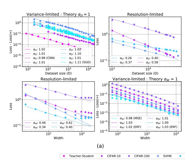
Empirical verification of variance-limited (exponent ≈ 1) and resolution-limited (exponent ≈ 0.26–0.62) regimes across Teacher-Student, CIFAR-10, CIFAR-100, and SVHN datasets.

Implications

This means that the Chinchilla coefficients broadly align with theoretical predictions in these one-dimensional infinite-limit settings.

But the major limitation remains: joint scaling in $N$ and $D$ , and especially scaling with interaction terms, is still not well explained by theory. That is why empirical construction still dominates practice.

Additionally, the assumptions behind the clean theory — local smoothness, effective convexity, manifold regularity — are not guaranteed in real deep networks. So in the real world, theoretical predictions for scaling coefficients are often unreliable, because quantities like the data manifold dimension are not known a priori.

Teacher–Student and Data Manifold Dimension

This is where scaling-law work becomes more physically interpretable.

The Sharma–Kaplan Dimension → Exponent Bridge

One influential idea (Sharma & Kaplan) is that scaling exponents can be explained by the intrinsic dimension of the data manifold. In that view, if neural models are effectively performing regression on a data manifold of intrinsic dimension $d$ , then the parameter-scaling exponent satisfies roughly

α \approx \frac{4}{d}

for cross-entropy and MSE losses.

This is interesting because it gives a "physical property" interpretation of the exponent: the exponent behaves like a critical exponent controlled by an effective dimension of the learning problem, not just by the fact that we are using Transformers.

Why Teacher–Student Matters

The teacher–student setup is useful because it gives a controlled environment where:

you can dial the teacher complexity,
you can vary the intrinsic dimension,
you can separate realizable vs non-realizable structure,
and you can measure how the fitted exponents move.

The point is not that teacher–student models are realistic LLMs. The point is that they let us identify what kind of hidden structure could generate the empirical exponents we later observe in real data.

A practical implication is that if you are building a scaling law for a new modality, it can be useful to first design synthetic teacher–student controls or procedural datasets to understand how geometry and complexity change exponents.

Compression, Zipf/Heaps, and Why $E$ Is Not "Just a Constant"

The compression-based perspective suggests a sharper interpretation of the irreducible term:

$E$ is closer to a code-length baseline for the evaluation distribution under the tokenizer.
Meanwhile the exponents and prefactors carry information about geometry, compressibility, and statistical complexity.

So the scaling-law coefficients are not merely fit parameters. They are often fingerprints of distributional structure plus training protocol.

Constructing Scaling Forms Beyond Dense-Text Transformers

Q1. Is Power Law Universal?

Empirically, power laws show up a lot, but "universal" is too strong. There are several concrete ways this fails.

Non-power-law transient regimes — Early training or small-data regions can look linear-ish or saturating before entering an asymptotic power-law regime.
Regime changes / bends / inflections — Broken or smoothly-broken power laws can be needed when multiple mechanisms are active.
Data selection changes the law — Better data pruning or curriculum can alter the apparent scaling with data size.

Vision Example: Why a Strict Power-Law Estimator Can Fail

One useful example from vision scaling laws is the distinction between fitting for interpolation vs fitting for extrapolation.

A common estimator is:

ε_{x} - ε_{\infty} = β x^{c}

This works if the observed points already lie in the asymptotic power-law regime. But when the data are not yet in that regime, a more flexible family is needed. One such corrected form is:

\frac{ε_{x} - ε_{\infty}}{(ε_{0} - ε_{x})^{α}} = β x^{c}

which reduces to the simpler saturating power law when $α = 0$ .

Excess risk estimator comparison: M2 vs M4
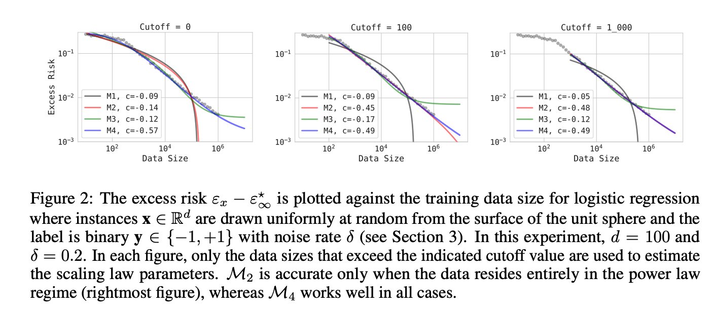
The excess risk $ε_{x} - ε_{\infty}^{*}$ plotted against training data size. M₂ (simple power law) is accurate only when data lies entirely in the power-law regime (rightmost panel), while M₄ (flexible form) works across all cutoff regimes.

The point is not that the power law is "wrong"; it is that a pure power law can fail if your observed regime is transitional.

Example: Exponential Law in Sparsity

In sparse-model work, one axis can empirically look exponential while another looks power-law. A representative form is:

L (N, S) = E + \frac{A (S)}{N^{α}}, A (S) = B + C \exp (\frac{β}{1 - S})

Sparse model scaling curves at fixed sparsity and fixed size
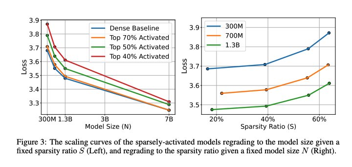
Left: scaling curves of sparsely-activated models vs. model size N at fixed sparsity ratio S. Right: loss vs. sparsity ratio at fixed N. Note the exponential behavior along the sparsity axis.

This is a good design pattern: if one dimension empirically looks exponential, do not force it into an additive $N^{- a} + D^{- b}$ template.

Q2. Are $N$ and $D$ the Only Dimensions to Consider?

For dense text-only models, people often treat "size" as parameter count and ignore shape, because upstream LM loss depends weakly on depth/width at fixed scale.

But this breaks quickly outside that setting.

In vision, compute-optimal performance can depend strongly on shape dimensions such as depth and width, and the compute-constrained loss can be quasiconvex in those axes.
In routed / MoE models, "model size" splits into total parameters vs active parameters per token vs routing structure.
In sparse / pruned models, sparsity ratio $S$ , non-zero parameter count, and active subnetwork size can matter directly.

Example: Vision Transformer Scaling

For vision transformers, the loss estimator proposed in Zhai et al. takes the form:

f_{k} (x_{k}, t) \sim α_{k} x_{k}^{- a_{k}} + (β_{k} x_{k}^{b_{k}} + ξ_{k}) t^{- c} + ε_{k}

When compute $t$ is unbounded, the loss follows a power law in the shape. This function is monotone and quasiconvex with respect to $x_{k}$ , which ensures a unique global minimum for the optimal shape at any compute budget. The power-law scaling exponent $c = Θ (1 / d)$ is governed by the intrinsic complexity of the data manifold.

So the answer is: no. $N$ and $D$ are not the only dimensions to consider. They are just the first two.

Q3. When to Include Interaction Terms?

The theory side does not provide guidance on when scaling coefficients couple across dimensions. The most practical recipe is:

Fit a separable form first.
Slice the data along one axis.
Check whether the fitted coefficients drift systematically with another axis.

If they do, your form is missing an interaction term.

Example 1: Routed / MoE Models

For routed models (Clark et al.), the first proposed scaling form is separable:

\log L_{N} (E) ≜ a \log N + b \log E + d

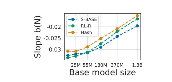
However, when fitting this form separately at each model size, the slope $b (N)$ with respect to experts drifts systematically with the base model size:

Slope b(N) drifts with base model size
The slope b(N) — the marginal benefit of adding more experts — is not constant; it grows (in magnitude) with base model size. This is the diagnostic for a missing interaction term.

The authors therefore propose the corrected form with an interaction term:

\log L (N, E) ≜ a \log N + b \log E + c (\log N) (\log E) + d

In log-space, multiplicative interactions are often the cheapest way to let one slope depend on another axis.

Example 2: Sparse Language Models (Frantar et al.)

When studying scaling laws for sparsely-connected foundation models, the sparse form needs to capture interaction between sparsity ratio $S$ , model size $N$ , and training tokens $D$ :

L (S, N, D) = (a_{S} (1 - S)^{b_{S}} + c_{S}) \cdot {(\frac{1}{N})}^{b_{N}} + {(\frac{a_{D}}{D})}^{b_{D}} + c

Visualizing the T5/C4 sweep results across all sizes and sparsity levels confirms the parallel structure:

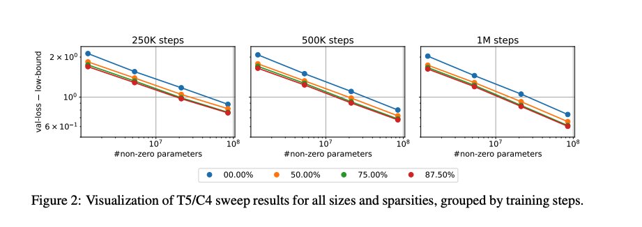
T5/C4 sweep: val-loss vs non-zero parameters at different training steps
Validation loss minus lower bound vs. number of non-zero parameters, grouped by training steps (250K, 500K, 1M). Loss vs. non-zero parameter curves for different sparsity levels form near-parallel lines — indicating that sparsity primarily shifts the A(S) prefactor.

Example 3: Alternative Sparse Form

A closely related form (from a different sparse LM paper) captures the sparsity dependence differently:

L (N, S) ≜ E + \frac{A (S)}{N^{α}}

where $α (S)$ should be non-decreasing in $S$ , and $A (S)$ is Lipschitz continuous with respect to $S$ .

Q4. Can We Have Multiple Scaling Forms for the Same Loss / Data Distribution?

Yes. There are usually several plausible forms to try:

additive vs multiplicative,
independent vs interacting,
power-law vs exponential,
single-regime vs broken-regime.

Several papers find that multiple fits can be similarly good in raw predictive accuracy. Then interpretability and parameter efficiency become real selection criteria.

A useful researcher mindset is that a scaling law is not just a fit. It is an extrapolator you trust under constraints.

Example 1: Scaling with Repeated Data

The scaling analysis for training with repeated data (Muennighoff et al.) compares multiple parametric fits. Chinchilla-style forms with no modification to account for data repetition have poor $R^{2}$ :

Comparison of parametric fits for repeated data scaling
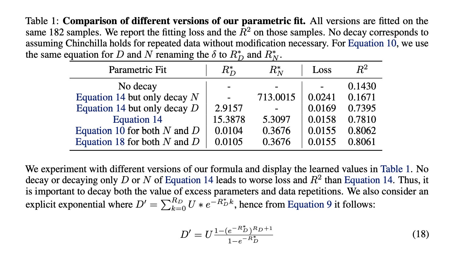
Table comparing different parametric fits. Forms that decay both the excess parameters and data repetitions (Equations 14, 10, 18) achieve R² > 0.80, whereas no-decay or single-axis decay forms are significantly worse.

This illustrates why it is important to introduce repetition explicitly into the law rather than absorbing it silently into $D$ .

Example 2: Data-Dependent Scaling Laws via Compressibility

The gzip data-dependent scaling law uses a two-step approach. First, define a compressibility score for each dataset:

H (D) = \frac{1}{∥ D ∥} \sum_{d \in D} \frac{∥ gzip (d) ∥}{∥ d ∥}

Then, fit the Chinchilla form separately for each dataset to obtain coefficients ${E, A, B, α, β}$ . Each coefficient is then predicted linearly from $H$ :

\forall x \in {E, A, B, α, β} : x (H) = m_{x} H + n_{x}

The final data-dependent scaling form is then:

L (N, D, H) = E (H) + \frac{A (H)}{N^{α (H)}} + \frac{B (H)}{D^{β (H)}}

A Practical Workflow for How Researchers Actually Come Up with Scaling Laws

This is the engineering reality.

Pick the metric and regime — Upstream next-token cross-entropy is often preferred because it is smooth and information-theoretically interpretable.
Define the axes precisely — What does $N$ mean? Non-embedding parameters? Total parameters? Effective active parameters? What does compute mean? Are embeddings and output head included? These choices matter.
Design the experiment grid around the question — If the question is compute-optimality, isoFLOP profiles and training-curve envelopes are central. If the question is shape-optimality, you need deliberate shape sweeps. If the question is sparsity, you need slices at different sparsity levels and training durations.
Fit for extrapolation, not just interpolation — A form that interpolates beautifully can extrapolate badly. Held-out extrapolation checks matter.
Look at coefficient drift — This is often the most informative diagnostic. If a "constant" changes systematically with another axis, your law is missing structure.

Where Scaling-Law Fits Go Wrong in Practice

A scaling-law project can fail because of things that look mundane:

schedule mismatch, especially when comparing models trained for different token budgets,
warmup effects,
optimizer / batch-size retuning across scales,
parameter-counting conventions,
data mixture changes,
tokenizer differences,
or simply fitting outside the asymptotic regime.

This is why it is better to think of a scaling law as a measurement protocol plus a functional family, not just an equation.

Off-Frontier Training and the LLM Reality Check

Overtraining Smaller Models Is a Scaling Axis in Its Own Right

A lot of real LLM practice does not live exactly on the Chinchilla frontier. Often we deliberately overtrain smaller models for more tokens to reduce inference cost.

This means the tokens-to-parameters ratio itself becomes a scaling variable of interest. In that setting, "compute-optimal" is not the only frontier that matters.

Repeated Data: When More Tokens Stop Meaning More Information

Once repeated data enters the picture, the mapping from "tokens processed" to "novel information acquired" bends.

So while Chinchilla-style $D$ is still fine as "tokens seen," if repeated tokens matter materially, then either:

you introduce repetition explicitly into the law,
or you accept that the effective data-scaling will bend or saturate.

Downstream Emergence and the Limit of Extrapolating from Loss

Another important LLM-era caution is that downstream metrics may show thresholds, inflections, or artifacts that do not inherit the smoothness of cross-entropy.

So if your real question is about downstream task performance, you should be careful about assuming that a clean upstream loss law transfers directly.

Final Takeaways

The Chinchilla form is best understood as a structured empirical ansatz, not a theorem.
The coefficients of a scaling law are often not arbitrary; they can reflect data geometry, compressibility, intrinsic dimension, and protocol choices.
The hardest and most important part of scaling-law work is usually choosing the right variables and the right experimental slices, not fitting the equation afterward.
Interaction terms should be added only after the data show you that separability fails.
Teacher–student settings, manifold-dimension arguments, and compression views are useful because they give a more "physical" interpretation of what the exponents might mean.
For LLMs, tokens processed, unique data, repeated data, data quality, and mixture composition are all distinct notions. Treating them as one variable can bias the fit.
A good scaling law is not just a curve fit. It is a reliable extrapolator for decision-making.

References

Kaplan et al., Scaling Laws for Neural Language Models.
Hoffmann et al., Training Compute-Optimal Large Language Models (Chinchilla).
Pearce et al., Reconciling Kaplan and Chinchilla Scaling Laws.
Sharma and Kaplan, A Neural Scaling Law from the Dimension of the Data Manifold.
Hutter, Learning Curve Theory.
Bahri et al., Explaining Neural Scaling Laws.
Alabdulmohsin et al., Revisiting Neural Scaling Laws in Language and Vision.
Alabdulmohsin et al., Getting ViT in Shape: Scaling Laws for Compute-Optimal Model Design.
Clark et al., Unified Scaling Laws for Routed Language Models.
Frantar et al., Scaling Laws for Sparsely-Connected Foundation Models.
Muennighoff et al., Scaling Data-Constrained Language Models.
Zhai et al., Scaling Vision Transformers.