Efficient continual pre-training of LLMs

I have been working on this topic on and off for some time now. While continual learning has been a subject of research for many decades now, I have been frustrated to see that most of these techniques cannot be adapted easily when pretraining language models on billions of tokens due to costly optimization procedure. So far, I haven't been able to materialize my research into any fruitful publication. Therefore, I decided to give a shot at trying to formulate the continual learning problem and propose few directions of research. This blog post will continue evolving over the next few weeks.

The objective of continual learning (CL) is to accumulate knowledge on non-stationary data or from a stream of non i.i.d. samples. Here I would discuss some methods that can be systematically applied for continual pretraining of LLMs. But CL for Large Language Models (LLM) is known to be limiting in its implementation in two scenarios: (1) the data for previous domains/tasks are assumed to be too large to start pretraining with all data from scratch (2) catastrophic forgetting of past information leading to the memorization vs generalization issue in pre trained language models. In that regard, there are two aspects of CL to focus on:

1. Backward Transfer: which is the influence that learning on a new domain has on the performance on downstream tasks of domains on which the LLMs were previously pretrained on. Positive backward transfer exists when learning about some domain increases the performance on tasks on some previously used domain. The opposite negative transfer is catastrophic forgetting.

2. Forward transfer: which is the influence that learning on a new domain has on the performance on downstream
tasks of domains on which the LLMs will be pretrained on, in future. This is the aspect of transfer learning or generalization that has been known to be an advantage of pre-trained LLMs.

One of the utilities of CL for LLMs is in developing a more principled approach to adaptive data selection strategies for sampling the replay buffer for CL as a sequential sampling problem or as a constrained optimization problem with speedup on large datasets and model sizes as well as for being better geared towards mitigating negative backward transfer. In that sense, there are many abstractions of the problem that can be formulated. Here, I provide a few forms of abstraction.

Abstraction I

Formally, we have a language model $M$ that has been trained on $D = {1, 2, 3 \dots}$ datasets, each of which has size $K_{d}$ , $d \in D$ and the total size of the data is $K = \sum_{d} K_{d} $ . An example would be - $D$ comprises datasets from 5 domains or 10 languages on which $M$ has already been trained on. We have a new dataset $T$ of one/many domains with size $R$ such that $R <<$ . We need to select examples or a subset $X \in D$ such that $∣ X ∣<< K$ that mitigates negative backward transfer while being able to achieve the domain improvement that comes along with training on $T$ . Here $R$ may be large (so for language models, they would be some several billion tokens), this differentiates it from intermediate low-resource pre-finetuning settings and post training model-editing with few examples, which is not the focus here. Additionally, we consider one aggregate dataset $T$ for now and $d$ can be fairly large.

Abstraction II

A different variant of this CL setup would be to select a subset $X \in D_{s u b}$ where $s u b$ denotes specific indices of the dataset $D$ (like choosing few datasets in $D$ ) along with $T$ , as we might want to continually adapt the model to only specific downstream tasks in the process of continual learning.

Yet a different variation of the learning problem can be as follows: we have a language model $M$ that has been trained on $D$ datasets, we have a new dataset $T$ of some domain. However, when training with $T$ , for some datasets $d^{'} \in D$ , we only have access to their validation data and the downstream task data related to $d^{'}$ , which would inhibit us from including $d^{'}$ in the replay buffer. The goal is use a mix of rehearsal on available data $D ∖ d^{'}$ and distillation/regularization in this case to mitigate forgetting.

Abstraction III

A tangential direction to handling the CL process is as follows: given a model with parameters $Θ = {θ_{l}}$ , $l$ denoting the layers in a model, the goal is to decompose $Θ$ into a shared parameter matrix $σ$ and a domain-adaptive parameter matrix $τ$ where the parameter matrix $σ$ is updated using $D$ and parameter matrix $τ$ is updated using $T$ . Note that this abstraction can be combined with the above three to improve the learning process.

A hard constrained continual learning would also entail constraints on the latency of the methods to enable a tradeoff between performance and time taken to adapt these models fast ( $L A T$ denoting the latency in either clock time or TFLOPS, $C$ being the corresponding value)

m i n_{σ, X :∣ X | \leq R} ​ E_{(x, y) \sim X} [L_{C E} (x, y, σ) ​] s . t . L A T (X) \leq C

Note: The following sections were initially drafted in 2023 as part of my exploration into continual pre-training methods. While some aspects may seem dated given the rapid progress in LLM research, the core principles and methodological approaches remain relevant.

Desiderata for the Problem

The problem statement defined in this proposal is close to multi-task pretraining with adaptive data selection and we want to improve on the sampling technique for data from different tasks while training.

Having defined the above abstractions, we lay out a few desiderata of the problem that applies to all of these abstractions:

We want to minimize negative backward transfer on downstream tasks related to $D$ but for each new task, we do not want to iterate over all of $D$ (which would be infeasible) and neither do we want to store or compute gradients offline/online over all of $D$ on the current or initial starting model. As an example, we might want to continually train multilingual models on topic specific corpuses like Covid corpus or a Twitter corpus in English. So for multilingual models, this means ensuring that language specific task performances do not degrade after the training. Additionally, we can also continually pretrain the language model with more data of one domain like tables or language like Egyptian Arabic so as to improve its performance, in that sense, the language or the tabular data becomes the new domain.
We want to avoid techniques like online batch selection during the CL process that solves a subset selection optimization problem for each mini-batch in an SGD optimization. This would not be feasible in terms of computation for large models and large data.
We want to avoid techniques like network expansion where possible, since these are often hard to adapt especially when we work with partner teams who have model size restrictions and specific model types to use. Also, most teams will have their own adapters for parameter-efficient finetuning so, adding our own adapters or prefixes like soft-prompts in the pre-training/pre-finetuning stage increases the complexity unless we have shared modeling plans across the teams.

What are Alternative CL Methods to Rehearsal?

Some details on methods alternative to rehearsal like generative replay, EWC have been listed in this review: Continually pretraining Multilingual LMs to alleviate forgetting. A different branch of work includes network expansion like adapters for domain specific finetuning, for example DEMIX Layers: Disentangling Domains for Modular Language Modeling which proposes mixture-of-experts to route specific FFN layers for specific domains and the recent work on Branch-Train-Merge, but these are parallel to rehearsal and could be taken up as a separate research direction for continual learning.

Evaluation Criteria

For each dataset $T$ of some domain on which $M$ is continually pretrained on, we have a corresponding related downstream supervised task $D_{C V}^{T}$ on which $M$ will be evaluated on. We want to measure the performance of $M$ on $D_{C V}^{T}$ before and after it is trained on $T$ in a zero-shot and few-shot manner. This will capture the impact of the CL technique on the new domain. Likewise, we want to measure the performance on tasks related to $D$ datasets before and after $M$ is trained on $T$ which will measure the forgetting aspect. Such evaluations are standard and have been done in similar works on CL.

Protocols for Learning

1. Single-Pass through All Data (Streaming)

Consider two streams of tasks, described by the following ordered sequences of datasets: $D_{C V} = {D_{1}, \dots, D_{T_{C V}}}$ and $D_{E V} = {D_{T_{C V} + 1}, \dots, D_{T}}$ where the first dataset is used for cross validation (hyperparameter selection) and the second dataset for training and evaluation. The training dataset can be replayed once and only once. The memory buffer for replay is usually fixed and there are some widely popular methods for updating the memory over the sequence: reservoir sampling, ring buffer, k-means, prototype exemplars.

2. Many Passes over All Data (Offline)

It is borrowed from supervised learning - during training the learner does as many passes over the data of each task $D_{E V} = {D_{T_{C V} + 1}, \dots, D_{T}}$ as desired. Moreover, hyper-parameters are tuned on the validation sets by sweeping over the whole sequence of tasks as many times as required by the cross-validation grid search. Finally, metrics of interest are reported on the test set of each task at the end of the training using the model selected by the previous cross-validation procedure. This setup is fairly similar to multi-task meta-learning where the goal is to quickly adapt to new datasets with few examples, however, considering that literature, the domain data $T$ is not small as is considered for few shot learning.

In this work we follow the second paradigm where we assume that the dataset $D$ is available for multiple passes. The second setup is quite similar to Curriculum Learning since we can control the sequence of the training data, however, for most practical purposes in pretraining, it is difficult to know what sequence to use since the downstream evaluation task data can be different from the pretraining data.

Baselines/Existing Work

What is the Simplest Baseline?

Given two sequential tasks A and B, there are two intuitive ways of training: (1) train on A and then train on B which will lead to forgetting the knowledge of A and then (2) train on A and then train on B but while regularizing using L2 norm. The below methods from well cited papers are some baseline experiments which I am exploring for a start.

B1. Mix-review

He et al.: Analyzing the Forgetting Problem in Pretrain-Finetuning of Open-domain Dialogue Response Models

In this work called Mix-review strategy, for each finetuning epoch, we mix the target data with a random subset $X$ of the pretraining data $D$ . This process introduces two hyper-parameters: mix-ratio, which controls how much pretraining data is mixed, and mix-decay, which decays mix-ratio by each epoch.

\begin{matrix} (1) & L_{X \cup T} = L_{T} (θ) + mix-ratio \cdot L_{X} (θ) \end{matrix}

It can be paired with an additional L2 regularization toward the pretrained parameters $L_{X} (θ) + λ \cdot ∥ θ - θ_{p r e} ∥$ . There can be different variants of this mixing process, where we can select the samples $X$ from $D$ for each epoch differently.

The simpler version of this is to keep mix-ratio to 1, but only use the loss $L_{X}$ every $t$ training steps.

B2. Logit Distillation

Methods like Dark Experience Replay alleviate forgetting by matching the network logits across a sequence of tasks during the optimization trajectory, formulated as below:

\begin{matrix} (2) & L_{D E R} = L_{T} (θ) + α \cdot E_{(x, p) \sim D} [∥ s o f t m a x (p) - s o f t m a x (h_{ψ} (x_{i}, τ)) ∥_{2}^{2}] \end{matrix}

where $p$ is the prob. of the target after the CL (step wise) and $h_{ψ}$ denotes the frozen network of $M$ prior to the CL process. This method has a disadvantage of blocking positive backward transfer where applicable (for example, continually training a pretrained multilingual model on more Portuguese data might not bring marginal improvements on this language), since the CL process will try to restrict the parameters towards the prior hypothesis class. This is also similar to regularization in the parameter space.

This method can be naturally extended to representation distillation where instead of matching the logits, match the layer parameters like the embedding layer or the last layer.

B3. Train on the Entire Data

The goal is to start fresh pretraining on the entire dataset $D \cup T$ . The method would not be feasible for the setting we have, as we consider pretraining with datasets where $K$ is large and especially for large model sizes. This is commonly referred to as the multi-task pretraining and while empirically, it should be better than the continual learning setup, sequential learning with replay can sometimes be better than MTL in that continual learning is hypothesized to often naturally provides a curriculum to models where each individual domain is easier to learn.

B4. Elastic Weight Consolidation

This used to be a very popular method for online/sequential continual learning and is an improved version of an L2 regularization but one that uses replay buffer. It is in a way a form of selective parameter updates as opposed to data selection we are proposing. Empirically, it has been observed that L2 regularization leads to degradation. EWC is a technique that updates the parameters when training on B while "selectively" adjusting the parameters that are important to A. Using the Fisher information from task A (which is where we use the replay buffer) denoted by $F_{A}$ , the optimization updates are as follows ( $θ_{A}$ being the optimal parameters prior to CL):

\begin{matrix} (3) & θ_{A, B} = \arg min_{θ} L_{B} (θ) + \frac{1}{2} \sum_{i} F_{i, i}^{A} (θ_{i} - θ_{i}^{A})^{2} \end{matrix}

This method is pretty neat, but it can take some computation overhead while computing the Fisher information on $D$ every minibatch for large datasets. There have also been known limitations of stability and the practical effectiveness of this method compared to naive rehearsal.

Proposed Methods/Experiments

The goal here is straightforward: we want/have to sample points from $D$ for the epochs, so the proposed experiments attempt at improving over uniform or random selection of replay examples especially for large datasets for each epoch. These methods can be extended to problems of continually training "undertrained model checkpoints" for more epochs but with sampled data that are selected through optimization.

E1: Probability Distributions for Sampling

Examples are sampled according to a multinomial distribution with probabilities ${q_{i}}_{i = 1}^{R}$ where $q_{i} = \frac{p_{i}^{α}}{\sum p_{i}^{α}}$ and $p_{i} = \frac{n_{i}}{\sum n_{i}}$ , $n_{i}$ denoting the # samples of the dataset to which $i$ belongs. This is essentially sampling based on the size of the datasets $d \in D$ in the pretraining corpus, $α$ determines the level of prioritization. When $α \to 0$ , then there is no prioritization, because all $p_{i} = 1$ . If $α \to 1$ , then we get to, in some sense, "full" prioritization, where sampling data points is more heavily dependent on the actual probabilities. Uniform sampling is a special case of this sampling procedure. There can be some variants of this approach where you can control how to tune $α$ over the epochs so as to put more emphasis on harder samples in the later stages of the learning.

The main disadvantage of this method is that the data selection is not tied to the optimization. So when we perform multiple rounds (like CL on the same model every 6 months) of continual learning on the same model, we may be using the same set of samples for every round which can at some point lead to overfitting. One way to alleviate this is to use an explore-exploit scenario so as to mix samples.

E2: Sequential (re)sampling of Memory Buffer

E3: Curriculum Learning for Adaptive Replay

E4: Select cR Examples from D and Use Dynamic Sampling

We adopt a hybrid between online optimization and offline sampling like E1. For the first epoch, train the model with $c R$ ( $c >> 1$ ) examples from $D$ (which we call $D^{'}$ ) which are randomly sampled (these could make use of E1 as well) and use them along with $T$ . Store the gradients of all the $c R$ examples in memory (or disk if it is too large). Thereafter we will train the model with $c^{'} R$ ( $c^{'} < c$ ) examples from $c R$ and all of $T$ for the rest of the epochs till convergence. However, every $g$ epochs, we select a different set of $c^{'} R$ examples from $c R$ based on an optimization criteria. The experiments proposed here are based on how we select $c^{'} R$ at every $g$ -th such epoch. Note that $c^{'}$ is a hyper-parameter that we fix beforehand, but this can also be tuned dynamically over the epochs based on some heuristics.

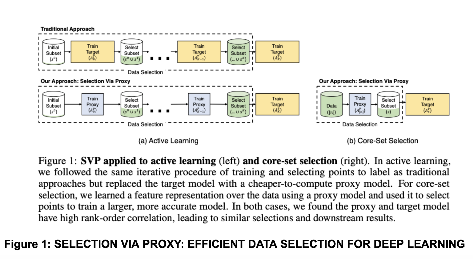
Before delving into the proposed experiments, we list down the existing approaches on adaptive data selection on which this work is based on. Adaptive data selection methods often do the data selection every $R$ epochs, so instead of running data selection every mini-batch in an SGD like optimization, the idea is to do offline selection prior to an epoch between some intervals. This has been the case for GradMatch where the data selection algorithm is run at intervals or for active learning scenarios where a proxy model is used to select points to then train a larger model as shown in the below figure.

Selection via Proxy: Efficient Data Selection for Deep Learning
Figure 1: Selection via Proxy - efficient data selection approach

The general philosophy of these data selection methods is based on coreset selections. Coresets are small and informative weighted data subsets that approximate original data in terms of some defined objective/metric (in our case, the distance between gradients). Several works have studied coresets for efficient training of deep learning models in the supervised learning scenarios. Although they have never been considered to be much in favor of training the models on full data for several days, these techniques seem relevant to our problem where we are necessitated to select a subset of data from $D$ that can mitigate negative backward transfer in the context of the new domain data.

The routine steps for such data selection methods are as follows:

Define an error function that you would want to use for selecting the points (these are standard gradient based errors). Here, selection means selecting a subset of the rehearsal data with weights every epoch or selecting a set of mini-batches in each epoch. An optimization algorithm will be able to select the data for you along with the weights. So the question boils down to the way you define the constraints to define the optimization objective and how the technique computes the associated weights.
Use some approximations to compute the gradients more efficiently like considering only last layer gradients and upper bounding gradient norm differences.
Solve the optimization problem such that we get $c^{'} R$ from $c R$ initial points to start with and each of the $c^{'} R$ points are associated with the weights. In our case, we may choose to ignore the weights.

Most of these methods are theoretically well studied in the context of convex functions where they assume Lipschitz continuity and smoothness to arrive at convergence rates and upper bound the errors. For our work, we mainly adapt these to our non-convex objective functions.

Why Cast Replay Buffer Selection as an Optimization Problem?

Most work on rehearsal till now have shown that rehearsal with random/proportional sampling works quite well, but they do not focus on situations where we need multiple rounds of CL (updates) on the same model. Simple rehearsal methods may end up repeating the same samples over the rounds, however, the logic behind sampling a fixed set of points for each $d$ in the replay buffer (like reservoir sampling) works well for the online setting and the bar for the offline setting is still low. Additionally, when $d$ (number of datasets) is large, we want our method to adaptively select the points from the datasets without worrying about the proportion to keep in our replay buffer every time and this proportion should be dynamic over the epochs.

Why Run First Epoch on All $c R$ Examples?

Warmstarting with large buffer has been known to help in many cases, in addition, we may want to do some importance sampling in the beginning and add some heuristics based on that for later sampling.

E2.1 GRAD-MATCH

GRAD-MATCH Procedure
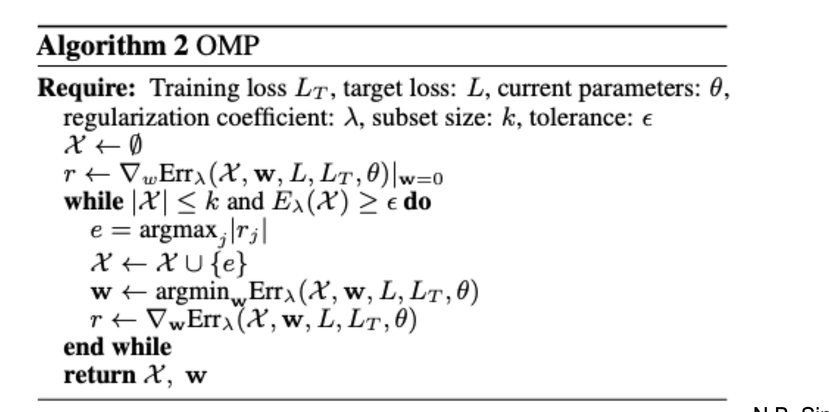
Figure 2: Procedure in GRAD-MATCH

The data selection optimization problem every $g$ epochs is as follows ( $t$ is the iteration number of this optimization step, $L$ is the training loss or the validation loss and $L_{T}$ is the training loss, $w$ denotes the weights of the selected points $X$ ):

\begin{matrix} (4) & w^{t}, X^{t} = \arg min_{w, X : | X | \leq c^{'} R} ‖ \sum_{i \in X^{t}} w_{i}^{t} \nabla_{θ} L_{T}^{i} (θ^{t}) - \nabla_{θ} L (θ^{t}) ‖ \end{matrix}

The norm is the L2 norm and the error is self-explanatory, difference between the gradient on all data points and the weighted coreset. We use norm of the gradient differences as the value since the goal is to approximate the full gradient with the coreset. These optimizations are solved using Orthogonal Matching Pursuit (OMP) algorithm (which are already included in many libraries) and are typically used to compute a greedy approximation to the solution of sparse coding problems in signal processing.

N.B. Since one of the steps of OMP include inverting the gradient matrix, we can do some approximations using Cholesky decomposition to speed the methods here. We also plan to do distributed greedy approximations across nodes in a map-reduce fashion so as to speed up the algorithm.

One of the key steps here is to achieve distributed computation of the signal recovery problem similar to distributed matrix factorization for speedups. For the 1st iteration of the experiments, we will consider separate optimizations and data selection for each node and there will be no communication between the nodes to reach a global solution to (4). Based on the experimental results, we may look into federated continual learning with inter-node communication for global optimization.

E2.2 Gradient Based Coreset Selection

Balles et al. 2022 extends the above approach to a more constrained setup in continual learning where we do not need the weights $w$ but we only need the subset, so in that sense the weights are binary masks (some are zeroed out and some that remain are kept for replay). The optimization is similar:

E_{p (θ)} = [{‖ \sum_{i = 1}^{c R} w_{i} \nabla l (θ; x_{i}; y_{i}) - \sum_{i = 1}^{c R} \nabla l (θ; x_{i}; y_{i}) ‖}_{2}]

subject to the cardinality constraint $∥ w ∥_{0} \leq c^{'} R$ , $c^{'} R$ is the desired coreset and $∥ w ∥_{0}$ denotes the pseudo-norm counting the number of non-zero entries in $w$ .

Approximations to speed up the method:

They project the embeddings $\nabla l (θ_{i}; x_{i}, y_{i})$ to a lower dimension than the # params (here $i$ is not a single point but a subset) using sparse random projection matrices
They use the last layer gradients when computing the gradients which is also a popular approximation adopted in many papers including GRAD-MATCH.

In my opinion, for large $K$ , we might want to keep the weights $w$ to be non-zero and select much fewer points as opposed to the formulation here where $w$ is binary, the reason being that we can keep $c^{'}$ to be small and use the weights to scale the loss from $X$ w.r.t. loss from $T$ .

E2.3 CRAIG (Coreset Selection)

The optimization problem of CRAIG is as follows:

\begin{matrix} (5) & S^{*} = \arg min_{S \subseteq V, γ_{j} \geq 0 \forall j} | S |, s.t. max_{w \in W} ‖ \sum_{i \in V} \nabla f_{i} (w) - \sum_{j \in S} γ_{j} \nabla f_{j} (w) ‖ \leq ϵ \end{matrix}

This optimization problem is particularly difficult to solve and they simplify it to:

\begin{matrix} (6) & S^{*} = \arg min_{S \subseteq V} | S |, s.t. \sum_{u \in V} min_{j \in S} max_{w \in W} ∥ \nabla f_{i} (w) - \nabla f_{j} (w) ∥ \leq ϵ \end{matrix}

where (6) is an upperbound to (5). It is still NP-Hard to solve it. The steps to solve this is:

Use a submodular function to approximate $∥ \nabla f_{i} (w) - \nabla f_{j} (w) ∥$ and then use a greedy hill climbing algorithm based on the submodular function to select the points till the subset size reaches end. This is widely popular for approximate solutions to NP-Hard problems as this one.
Once the subset (coreset) is selected, the weights are defined by the nearest points (similar to k-medoids) in the entire data to these coresets.

The main drawback with this approach is the greedy submodular algorithm for selecting the coreset. It is expensive for coreset selections among millions of points.

E2.4 Our Method v1

Since most of these methods are not adapted to continual learning, the data selection through optimization is separate from the training process. We want to select the subset $X \in D^{'}$ while keeping the gradient calculations in the context of target domain $T$ . Based on the above methods E2.1 and E2.2, the steps for the selection is as follows: at the start of the $g$ -th epoch, we will select the points by optimizing the following objective:

\begin{matrix} (7) & w^{t}, X^{t} = \arg min_{w, X : | X | \leq c^{'} R, X \in D^{'}} [‖ \sum_{i \in X} w_{i} \nabla l (θ; x) - (\sum_{j \in D^{'}} \nabla l (θ; x_{j}) + \sum_{k \in T} \nabla l (θ; x_{k})) ‖] \end{matrix}

subject to the cardinality constraint $∥ w ∥_{0} \leq n$ , where $n << c R$ and $n$ is the desired coreset size and $∥ w ∥_{0}$ denotes the pseudo-norm counting the number of non-zero entries in $w$ (as mentioned, we will also experiment without the pseudo-norm constraint). We will apply the same approximations as done in other methods to speed up the computations, some of which are described above.

Some considerations:

Mini-batch subsets - since we generally consider points in the context of mini-batches, the problem can reformulated as selecting mini-batches among a set of mini-batches instead of single points in an epoch. This will speed up the gradient computations by a factor.
Multi-node computations - Since we use multi-node sharding of pretraining data, the speedup can also come from more efficient techniques to shard the data offline based on importance sampling.

E2.5 Our Method v2

As mentioned in the problem statement, since our data has $D$ datasets, each of which has size $K_{d}$ , $d \in D$ , we want to experiment with local data selection, where by local we mean, run the optimization problem in E2.4 but separately for each dataset $d \in D$ and then concatenate the selected subset of datasets for rehearsal.

E2.6 Our Method v3

This is similar to meta-learning where the model is trying to jointly learn which examples to pick and learn how to update the model parameters following that. A different method would be to do a bi-level optimization similar to the approach used in Safe Deep Semi-Supervised Learning for Unseen-Class Unlabeled Data. We can do a one step gradient optimization of the network considering $D \cup T$ and use this new parameter set as a starting point to optimize on $T$ . So the optimization problem is as follows:

X = \arg min_{X : | X | \leq c^{'} R, X \in D^{'}} L (T, \arg min_{θ} (L_{T} (θ) + mix-ratio \cdot L_{D^{'}} (θ)))

The inner level optimization is only run for 1 gradient step on the entire pretraining corpus. This requires solving a discrete optimization for the outer level problem. This will be explored as a separate research problem.

Speeding up the Optimization in Eq. 7

The goal is to carry out importance sampling with distributed training as an independent step similar to techniques used in variance reduction techniques for SGD - Not All Samples Are Created Equal: Deep Learning with Importance Sampling. One example from Variance Reduction in SGD by Distributed Importance Sampling provides relevant techniques.